
A Wavelet Scattering Convolutional Network for Magnetic
Resonance Spectroscopy Signal Quantitation
Amirmohammad Shamaei
1,2 a
, Jana Starčuková
1 b
and Zenon Starčuk Jr.
1 c
1
Institute of Scientific Instruments of the CAS, Královopolská 147, 612 64 Brno, Czech Republic
2
Department of Biomedical Engineering, Faculty of Electrical Engineering and Communication,
Brno University of Technology, Technická 3058/10, 616 00 Brno, Czech Republic
Keywords: Magnetic Resonance Spectroscopy, Quantification, Deep Learning, Machine Learning.
Abstract: Magnetic resonance spectroscopy (MRS) can provide quantitative information about local metabolite
concentrations in living tissues, but in practice the quantification can be difficult. Recently deep learning (DL)
has been used for quantification of MRS signals in the frequency domain, and DL combined with time-
frequency analysis for artefact detection in MRS. The networks most widely used in previous studies were
Convolutional Neural Networks (CNN). Nonetheless, the optimal architecture and hyper-parameters of the
CNN for MRS are not well understood; CNN has no knowledge about the nature of the MRS signal and its
training is computationally expensive. On the other hand, Wavelet Scattering Convolutional Network
(WSCN) is well-understood and computationally cheap. In this study, we found that a wavelet scattering
network could hopefully be also used for metabolite quantification. We showed that a WSCN could yield
results more robust than QUEST (one of quantitation methods based on model fitting) and the same as a CNN
while being faster. We used wavelet scattering transform to extract features from the MRS signal, and a
superficial neural network implementation to predict metabolite concentrations. Effects of phase, noise, and
macromolecules variation on the WSCN estimation accuracy were also investigated.
1 INTRODUCTION
Magnetic Resonance Spectroscopy (MRS) has
attracted the MR community over the past seven
decades (Van Der Graaf, 2010). A significant part of
the interest in biomedical MRS stems from the
possibility of noninvasive measurements of
metabolites. Information about tissue metabolites can
help in clinical diagnostics. For instance, detection of
metabolic pathway changes may facilitate diagnosing
disease in earlier stages before anatomy changes can
be observed, and thus enable more efficient treatment.
E.g., in glioma, a decrease of N-acetylaspartate
(NAA) and creatine concentrations and an increase of
choline, lipids, and lactate predicts an increase of the
glioma grade (Robin A. de Graaf, 2019; Van Der
Graaf, 2010). To detect such changes, quantification
of MRS signals is required for obtaining the
metabolite concentrations in the tissue. However,
a
https://orcid.org/0000-0001-8342-3284
b
https://orcid.org/0000-0003-0337-7893
c
https://orcid.org/0000-0002-1218-0585
reliable quantification of MRS is difficult. The
existing MRS quantitation methods are based on
model fitting of the signal in either the time or the
frequency domain (Poullet et al., 2008). In recent
years, new novel machine learning solutions have
been proposed for quantification, one of which is
deep learning (DL). Even though the first usage of
machine learning dates back to the 1970s, it was
unpractical until the past decade due to lack of high-
performance hardware and novel algorithms (Chen et
al., 2020). DL has achieved many accomplishments
in a wide range of tasks, including the MRI field
(Alaskar, 2019). Due to the poor SNR, chemical shift
displacement, and overlapping signal components in
MRS signals, only recently has DL been used for
metabolite quantification of MRS signals in the
frequency domain (Hatami et al., 2018; Lee & Kim,
2019)
268
Shamaei, A., Star
ˇ
cuková, J. and Star
ˇ
cuk Jr., Z.
A Wavelet Scattering Convolutional Network for Magnetic Resonance Spectroscopy Signal Quantitation.
DOI: 10.5220/0010318502680275
In Proceedings of the 14th International Joint Conference on Biomedical Engineering Systems and Technologies (BIOSTEC 2021) - Volume 4: BIOSIGNALS, pages 268-275
ISBN: 978-989-758-490-9
Copyright
c
2021 by SCITEPRESS – Science and Technology Publications, Lda. All rights reserved

Hatami et al. showed the first step in this area by
using the Convolutional Neural Network (CNN)
approach for simulated MRS signal quantification
(Hatami et al., 2018). Kim et al. conducted a
comprehensive study on brain metabolite
quantification using DL (Lee and Kim, 2019).
Nonetheless, the practical application of DL in MRS
has not been limited to quantifications only.
Kyathanahally et al. taught a CNN with time-
frequency data to detect and remove ghosting artifacts
in clinical magnetic resonance spectra of the human
brain (Kreis & Kyathanahally, 2018).
However, the optimal architecture and hyper-
parameters of CNN for MRS are not well understood.
Besides, training a CNN is a computationally
expensive and time-consuming task, and it usually
needs a big dataset (Bruna & Mallat, 2013).
Moreover, in the case of MRS signals, CNN has no
understanding of the nature of the signal, and
therefore, any shape difference of the signal under
investigation from signals in the training data set can
lead to CNN failure. If we look at a CNN as a
transformation from the time domain to a features
domain, due to the nature of MRS signals, the
transformation should be invariant to time shift,
deformation in the time domain, and frequency shift.
To satisfy such requirements, CNN could be designed
as
- an optimized and simple deep architecture
which pools the features using a nonlinear averaging
measure.
- a network with a fast computational
algorithm which is stable to time-shifting,
deformation in the time domain, and frequency shift.
Wavelet Scattering Convolutional Network
(WSCN) can be a method of choice. WSCNs are
well-understood, computationally cheap, and fast for
a deep learning task (Andén & Mallat, 2014; Bruna &
Mallat, 2013). Wavelet-based methods have
previously been used for MRS quantification and
water removal (Poullet et al., 2008; Suvichakorn et
al., 2008); but as far as we are aware, wavelet
transform has not been implemented by a deep
convolutional neural network to quantify MRS
signals.
Given the mentioned accomplishments of
machine learning in MRS for signal quantification,
this paper describes to our knowledge the first attempt
to use this state-of-the-art technique to quantify MRS
signals by WSCNs. We used wavelet scattering
transform to extract features from the free induction
decay (FID, i.e. the MRS signal in the time domain)
and a superficial neural network implementation to
predict metabolite concentrations.
In this study, we used two different basis sets. The
first basis set was the ISMRM challenge 2016
simulated basis set for comparing results of our
method with the results published for a CNN and
another conventional quantification method, QUEST
(Graveron-Demilly, 2014). For the second basis set,
we simulated our own metabolite signals and
generated different synthetic datasets from them for
evaluating our method against phase changing, noise,
and presence of macromolecule signals.
2 METHODS
All steps were run on a laptop with a 4-core Intel i7
processor running at 2.6 GHz and an NVIDIA GTX
1050Ti graphics processing units using Matlab
(R2019a, Mathworks Inc., Natick, MA, USA)
software.
2.1 Simulation of Metabolites
To build a basis-set signals, fifteen metabolites –
Alanine (Ala), Aspartate (Asp), Creatine (Cr),
Choline (Cho), Gamma Aminobutyric Acid (GABA),
Glutathione (GSH), Glutamine (Gln), Glutamate
(Glu), Lactate (Lac), N-Acetylaspartate (NAA), N-
acetyl-aspartyl-glutamate (NAAG), Phosphatidyl-
choline (PC), Phosphocreatine (PCr), Taurine (Tau)
and myo-Inositol (mIns) – were simulated at 9.4 T
magnetic field with the PRESS sequence (TE = 20
ms; TR = 2500 ms; acquisition points: 2048;
acquisition bandwidth: 4401.41 Hz; three PRESS
pulses with Hermite shapes and flip angles: P1 = 90°,
P2 = 180°, P3 = 180°). The simulation was performed
in NMRScopeB (Starčuk & Starčuková, 2017; Stefan
et al., 2009). The parameters selected in the sequence
were taken from an in-vivo experiment, which allows
reusing the simulated basis set.
2.2 Baseline and Macromolecule
Simulation
The baseline signals were simulated as a linear
combination of several Gaussian lines identified by
Osorio-Garcia (Opstad et al., 2008; Osorio-Garcia et
al., 2011). The number and parameters of Gaussian
lines were extracted from in-vivo signals using
inversion recovery (Osorio-Garcia et al., 2011).
2.3 Signal Generation Framework
The MRS signal was defined as a linear combination
A Wavelet Scattering Convolutional Network for Magnetic Resonance Spectroscopy Signal Quantitation
269

of amplitude-scaled frequency- and phase-shifted
metabolite signals, the baseline, and noise.
The model describing a time-domain MRS signal
s[n] as a combination of several metabolite profiles is
(Poullet et al., 2007):
n
nMMA
nXAns
MMMMMM
mmm
itnfi
MM
itnfi
M
m
mm
+
++
+=
+
+
=
ee
ee
)2(
)2(
1
(1)
where
is the n-th sample of the m-th simulated
metabolite, is the sampling period, A
m
is the
scaling factor of the metabolite,
m
is the damping
factor, Δf
m
is the frequency shift of the m-th
metabolite affected by the static magnetic field
inhomogeneity, pH, temperature and chemical
composition of the tissue,
is the phase of the m-
th metabolite, Δt is the time step, and M is the number
of metabolites.
Table 1 specifies the range of parameter values
used for generating different datasets according to
equation (1). For a comparison of our results with the
previous study (Hatami et al., 2018), the basis set
provided for the ISMRM challenge 2016 (ISMRM,
2016) was used to generate dataset DSS1 (20
metabolite and one macromolecule components). All
other datasets were generated using the basis set
simulated with NMRScopeB (15 metabolites). The
same parameter ranges that were used in the previous
study (Hatami et al., 2018) were also used in this
study for DSS1, but we decided to choose ranges of
parameters for other datasets (DSS2-DSS7) in the
same manner as we would do if we evaluated real
acquired spectra.
Instead of generating 500 000 signal samples per
dataset, in our study only 10 000 signal samples were
generated for validating the hypothesis that our
network is as robust as Hatami et al.'s approach
(Hatami et al., 2018) even with a smaller number of
samples but faster. Parameters were chosen randomly
from defined ranges with a uniform distribution. In
DSS1, random complex Gaussian noise was added to
signal samples based on the previous study (Hatami
et al., 2018). In the rest of the datasets, the SNR of the
signal samples was adjusted by adding random noise
such that the SNR was in the range of ~5 to ~15. In
this study, we used MATLAB built-in snr function
which calculates the signal-to-noise ratio (SNR) of an
MRS signal by computing the ratio of its summed
squared magnitude to that of the noise. In Table 1, the
presence of a parameter is marked by a tick and the
absence of a parameter by a cross.
2.4 Deep Learning
2.4.1 Invariant Wavelet Scattering Network
Invariant wavelet scattering network is a transform
from the time domain to the features domain, which
has three stages, namely, Convolution (wavelet),
Non-linearity, and Averaging (scaling factor).
In contrast to the classical wavelet transform, the
Complex wavelet transform is translation invariant.
In this study, we chose Morlet (Gabor) wavelets, a
type of complex wavelet transform, because they
have a simple mathematical representation.
Figure 1 illustrates the wavelet scattering
transform processes (see (Andén & Mallat, 2014;
Bruna & Mallat, 2013) for more details). In practice,
a scattering decomposition framework was created
with a signal input length of 1024 samples.
Table 1: Specification of datasets.
Name
Amplitude
(A
m
)
Frequency
shift(Δf
m
)
Damping
range(
m
)
Noise
()
Phase (
)
MM (
)
Common
Separated
Constant
Changing
DSS1
(Hatami et
al., 2018)
[0, 1]
[-10, 10]
[-10, 10]
DSS2
[0.5 1]
[-10, 10]
[-5, 2.5]
DSS3
[0.5 1]
[-10, 10]
[-5, 2.5]
[
]
DSS4
[0.5 1]
[-10, 10]
[-5, 2.5]
[
]
DSS5
[0.5 1]
[-10, 10]
[-5, 2.5]
[
]
DSS6
[0.5 1]
[-10, 10]
[-5, 2.5]
DSS7
[0.5 1]
[-10, 10]
[-5, 2.5]
Within ±10 percent
of initial values
BIOSIGNALS 2021 - 14th International Conference on Bio-inspired Systems and Signal Processing
270
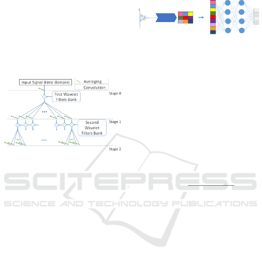
The framework had two filter banks; in other words,
the depth of the framework was 3. The quality factor
(the number of wavelet filters per octave) of the first
and second filter banks were 8 and 1, respectively.
For the given signal length and quality factors, the
output of the framework was a matrix with a size of
154 by 8 by 2. There were 154 scattering paths and 8
scattering windows for each of the real and imaginary
parts of the signal.
2.4.2 Regression
Figure 1: The process of wavelet scattering network;
averaging and convolution of a signal with wavelet filters
are showed by an arrow (green) and a circled star,
respectively.
Flattening and fully-connected layers were what we
had at the last stage of our network. The first step, so-
called flattening, was converting a feature matrix into
a 1-dimensional array. The matrices from the output
of WSCN were flattened to create a single long
feature vector. The flattening layer was connected to
a fully-connected layer, which was a feedforward
artificial neural network for the regression task.
Neural networks with the different number of neurons
in hidden layers were investigated. The best fully-
connected layer structure was obtained by trial and
error on the basis of the lowest error on the training
and validation dataset. The results showed that one
hidden-layer network with 20 neurons in the hidden
layer yielded better results than other network types.
The modeling performance and training were
evaluated by the mean square error (MSE) and scaled
conjugate gradient, respectively.
Figure 2 demonstrates the process of
transformation, flattening, and regression. The input
and output of a fully-connected layer were the
features vector and the relative amplitudes of various
metabolite basis spectra, respectively.
Figure 2: A schematic of feature extraction and flattening
and the training of an artificial neural network.
2.4.3 Quantification
80% of each dataset was allocated to the training set,
10% for validation and the rest 10% for the test set. It
applied to all datasets, DSS1 to DSS7, and then they
were fed to the network. First, the network was
trained with the training dataset; then, it was used to
predict the test dataset. The output of the network was
a vector in which each element represents the relative
amplitude of each metabolite.
2.5 Accuracy Evaluation
The Symmetric mean absolute percentage error
(SMAPE) is used to measure the accuracy of the
model. SMAPE is defined as below for each
metabolite:
′
′
(2)
Where m, N, A, and
′
are the metabolite index, the
number of test datasets, the ground truth, and the
estimated amplitude, respectively.
3 RESULTS
3.1 Comparison between the
Quantification Result of QUEST,
CNN, and WSCN for ISMRM
Challenge Dataset
Figure 3 shows the comparison between different
methods, namely Quest, CNN, and WSCN, for
dataset DSS1, where the SNR of signals was set to 10.
The result for CNN and QUEST were extracted from
(Hatami et al., 2018).
Flattening
Feature
Extraction
Signal(s[n])
A Wavelet Scattering Convolutional Network for Magnetic Resonance Spectroscopy Signal Quantitation
271
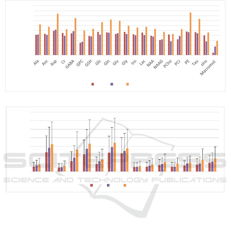
Figure 3: Comparison between SMAPEs of each metabolite for the WSCN (red), the CNN (yellow), and Quest (green).
Figure 4: Comparison between SMAPEs of the concentration of all metabolites with fixed phases (DSS2), common phase
varied (DSS3) and independently varied phases (DSS4) (different phase changes for different metabolites). (Test datasets,
N=1000). The error bars represent the standard deviation.
3.2 Effect of Phase Variation and Noise
on WSCN Estimation Accuracy
The performance of WSCN was evaluated on
different datasets (DSS2 to DSS7) in table 1. Figure
4 shows the effect of metabolite phase variation in the
signals under test. We compared the result of signals
with a fixed phase, a common varied phase, and
independently varied phases. The average of
SMAPEs for DSS2, DSS3, and DSS4 were 1.13%,
1.38%, and 1.7%, respectively.
The results of the metabolite quantification for
DSS5 (DSS3 with added noise) is shown in Figure 5.
For all 15 metabolites, the average of SMAPE was
3.46% ± 2.81%. Asp with SMAPE of 6.00 ± 4.48 and
NAAG with SMAPE of 13.20% ± 10.12% were
quantified as highest and lowest SMAPE,
respectively. The average SMAPE of DSS5 was
increased by 151% compared to DSS3 (without
noise).
3.3 Effect of Macromolecules Variation
on WSCN Estimation Accuracy
Figure 6 shows a comparison between DSS6 and
DSS7. In dataset DSS6, the parameters of baseline
signals (11 Gaussian lines) are constant, while in
DSS7, amplitudes of Gaussian lines were randomly
varied in the range of ±10% of their initial values. For
all metabolites of DSS6 and DSS7, the average
SMAPEs were 5.92% ± 4.40% and 6.12% + 4.55%,
respectively. The average SMAPE of DSS6 and
DSS7 was increased by 73% compared to DSS5
(without Macromolecules inclusion).
0
5
10
15
20
25
30
35
40
45
50
Symmetric mean absolute
percentage error (SMAPE, %)
WSCN CNN Quest
0
1
2
3
4
5
6
7
Ala Asp Cr Cho GABA GSH Gln Glu Lac NAA NAAG PC PCr Tau mIns
Symmetric mean absolute
percentage error (SMAPE, %)
DSS2 DSS3 DSS4
BIOSIGNALS 2021 - 14th International Conference on Bio-inspired Systems and Signal Processing
272
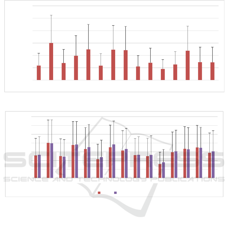
Figure 5: Symmetric mean absolute percent error (SMAPE) of the concentrations of all metabolites in dataset DSS5, which
contains noisy signal (N = 5000). The error bars represent the standard deviation.
Figure 6: Comparison between SMAPEs of the concentration of all metabolites in dataset DSS6, and DSS7 (Test datasets,
N=1000). In DSS6, the amplitudes of macromolecules lines were constant. In contrary, the amplitudes were varying within
±10% of initial range in DSS7. Both datasets are noisy and with common phase changing.
4 CONCLUSIONS
The aim of MRS signal quantification is to estimate
the amplitudes/areas (in time/frequency domain) of
different metabolites in the signal. The estimated
amplitudes/areas then can be converted to meaningful
numbers as the concentration of metabolites. The
conventional and widely used approach is to estimate
amplitudes of single sinusoids (areas of single peaks)
in MRS signal or to estimate the amplitudes (areas) of
whole metabolite signals (spectra). In the former
approach, the model is fitted to data using non-linear
least-squares analysis; the latter approach uses a basis
set of metabolite profiles in the model function and
uses a semi-parametric fitting technique. The oldest
method, so-called peak integration, is calculating
peaks area in a selected frequency interval.
Nonetheless, using these approaches for
quantification is challenging (Stagg & Rothman,
2014).
On the other hand, the quantification of the MRS
signal using deep learning has attracted huge interest
in recent years (Chen et al., 2020). DL can detect
important features in the MRS signal and
subsequently determine a non-linear mapping
between these features and the outputs, which can be
the concentrations of the metabolites. The most
widely used DL approach for quantification is CNN.
Nevertheless, this approach has drawbacks, for
example, poor understanding of the CNN architecture
and hyper-parameters for MRS, expensive and time-
0
2
4
6
8
10
12
Ala Asp Cr Cho GABA GSH Gln Glu Lac NAA NAAG PC PCr Tau mIns
Symmetric Mean absolute
percentage error (SMAPE, %)
0
2
4
6
8
10
12
14
Ala Asp Cr Cho GABA GSH Gln Glu Lac NAA NAAG PC PCr Tau mIns
Symmetric mean absolute
percentage error (SMAPE, %)
DSS6 DSS7
A Wavelet Scattering Convolutional Network for Magnetic Resonance Spectroscopy Signal Quantitation
273

consuming computation, and the need of a big dataset
for CNN training (Bruna and Mallat, 2013).
These shortages motivated us to develop a deep
network for MRS signal quantification, which can be
fast, well-understood, and works with a small dataset
of training samples. For this purpose, we used a
WSCN.
In every DL task, determining the proper input
and output of the network is an important step. In our
study, the input is an FID, i.e., time-domain signal,
and the network estimates amplitudes of the first
points of metabolite signals (what corresponds to
areas under metabolite signals in metabolite spectra).
In this work, we demonstrated that the use of the
wavelet scattering network could achieve better
results than the semi-parametric fitting technique
QUEST and similar results as the computationally
more demanding CNN (Figure 3).
It is known that the accuracy of estimation in the
peak integration approaches is influenced by phases
of peaks (Stagg & Rothman, 2014), and that phase
should be included in the model as one of the
unknown parameters. Therefore, we also investigated
whether WSCN is capable of estimating amplitudes
of metabolites in case that metabolite phases change.
It resulted in an increase in the complexity of the
model, but WSCN proved to have the capability of
handling this task. Figure 4 shows the WSCN can
quantify signals with common varied phases (with
SMAPE of 1.38%) as well as signals without fixed
phases (with SMAPE of 1.13%). The average of
MAPEs for DSS4 is increased by 36% and 17%
compared to DSS2 and DSS3, respectively. It
indicates that quantification can be moderately harder
for a dataset with independently varied phases.
Another source of error in quantification are
macromolecular signals, which stem in macro-
molecules present in the tissue under investigation. In
conventional quantification approaches, macro-
molecule signals can either be removed in the
preprocessing step or modeled in the quantitation
step. However, the risk of errors will be increased and
accumulated in fitting error in the former approach,
and therefore the latter approach is recommended.
However, macromolecule signals often overlap with
metabolite components, for which DL can be a
method of choice for disentangling. As we showed in
Figure 3, the WSCN could estimate macromolecules
better than other approaches. Later in this study, we
modeled the macromolecules signal as a set of
Gaussian lines using parameters (like linewidth,
frequency) measured using the inversion-recovery
recovery (Osorio-Garcia et al., 2011). Figure 6
demonstrates that the WSCN showed nearly the same
error for signals with randomly varied macro-
molecule lines and signals with fixed macromolecule
lines. This could indicate that despite the changing of
background signals parameters, the WSCN is stable
against nuisance components in MRS, such as
macromolecules. Additional research should be done
however with simulated signals that will imitate in-
vivo data.
To compare the learning times of both networks,
i.e., Hatami et al.'s CNN and our WSCN, we rebuilt
their CNN and fed both networks with the DSS5
dataset, and ran both networks in the earlier
mentioned system. Our proposed approach is
estimated to be 45 times faster than Hatami et al.'s
approach (the WSCN’s learning time was 5 min 40
sec precisely and the CNN’s learning time was 268
min). The WSCN showed that it could be faster than
the CNN due to using fixed-size filters and less
parameter optimization.
It should be noted that even though deep learning
showed promising results in areas like speech
recognition and image processing (Chen et al., 2020),
this study is one of the very initial steps in the
application of DL in MRS and more studies are
needed for proving DL suitability for in-vivo
spectroscopy. Below some of the limitations and open
issues are addressed:
1. In this study, we only quantified simulated
data. The amplitudes of metabolites in our
simulated data did not imitate the metabolite
concentrations in in-vivo data. Quantification of
simulated data with concentrations close to in-
vivo data should be investigated as the next step
together with data acquired from a phantom.
2. Real MRS data is influenced by numerous
factors such as voxel size, voxel placement,
radiofrequency (RF) coil sensitivity, receiver
gain, and other experimental factors. Further
research must take all factors into account.
3. A potential application of our proposed
approach is the quantification of MRSI data,
where a fast method is needed for quantification
of a set of MRS signal. Learning a network and
using it for only a single voxel may not be
efficient as using it for a set of signals.
ACKNOWLEDGEMENTS
This research was supported by European Union's
Horizon 2020 research and innovation program under
the Marie Skłodowska-Curie grant agreement No
813120 (INSPiRE-MED) and by European Regional
Development Funds under project "National
BIOSIGNALS 2021 - 14th International Conference on Bio-inspired Systems and Signal Processing
274

infrastructure for biological and medical imaging" of
the Ministry of Education, Youth and Sports of the
CR (No. CZ.02.1.01/0.0/0.0/16_013/0001775).
REFERENCES
Alaskar, H. (2019). Deep Learning-based Model Architec-
ture for Time-Frequency Images Analysis. January
2018.
Andén, J., & Mallat, S. (2014). Deep scattering spectrum.
IEEE Transactions on Signal Processing, 62(16),
4114–4128.
Bruna, J., & Mallat, S. (2013). Invariant scattering
convolution networks. IEEE Transactions on Pattern
Analysis and Machine Intelligence, 35(8), 1872–1886.
Chen, D., Wang, Z., Guo, D., Orekhov, V., & Qu, X.
(2020). Review and Prospect: Deep Learning in
Nuclear Magnetic Resonance Spectroscopy. Chemistry
- A European Journal, 26(46), 10391–10401.
Graveron-Demilly, D. (2014). Quantification in magnetic
resonance spectroscopy based on semi-parametric
approaches. In Magnetic Resonance Materials in
Physics, Biology and Medicine (Vol. 27, Issue 2, pp.
113–130). Springer Verlag.
Hatami, N., Lyon, B., & Etienne, U. (2018). Magnetic
Resonance Spectroscopy Quantification using Deep
Learning.
ISMRM. (2016). MRS Fitting Challenge (ismrm.org
/workshops/Spectroscopy16/mrs_fitting_challenge/).
Kreis, R., & Kyathanahally, S. P. (2018). Deep Learning
Approaches for Detection and Removal of Ghosting
Artifacts in MR Spectroscopy. 863, 851–863.
Lee, H. H., & Kim, H. (2019). Intact metabolite spectrum
mining by deep learning in proton magnetic resonance
spectroscopy of the brain. Magnetic Resonance in
Medicine, 82(1), 33–48.
Opstad, K. S., Bell, B. A., Griffiths, J. R., & Howe, F. A.
(2008). Toward accurate quantification of metabolites,
lipids, and macromolecules in HRMAS spectra of
human brain tumor biopsies using LCModel. Magnetic
Resonance in Medicine, 60(5).
Osorio-Garcia, M. I., Sima, D. M., Nielsen, F. U.,
Dresselaers, T., Van Leuven, F., Himmelreich, U., &
Van Huffel, S. (2011). Quantification of in vivo 1H
magnetic resonance spectroscopy signals with baseline
and lineshape estimation. Measurement Science and
Technology, 22(11), 1–17.
Poullet, J. B., Sima, D. M., Simonetti, A. W., De Neuter,
B., Vanhamme, L., Lemmerling, P., & Van Huffel, S.
(2007). An automated quantification of short echo time
MRS spectra in an open source software environment:
AQSES. NMR in Biomedicine, 20(5), 493–504.
Poullet, J. B., Sima, D. M., & Van Huffel, S. (2008). MRS
signal quantitation: A review of time- and frequency-
domain methods. Journal of Magnetic Resonance,
195(2), 134–144.
Robin A. de Graaf. (2019). In Vivo NMR Spectroscopy. In
In Vivo NMR Spectroscopy (pp. 1–42).
Stagg, C., & Rothman, D. (2014). Magnetic Resonance
Spectroscopy: Tools for Neuroscience Research.
Starčuk, Z., & Starčuková, J. (2017). Quantum-mechanical
simulations for in vivo MR spectroscopy: Principles
and possibilities demonstrated with the program
NMRScopeB. Analytical Biochemistry, 529.
Stefan, D., Cesare, F. Di, Andrasescu, A., Popa, E.,
Lazariev, A., Vescovo, E., Strbak, O., Williams, S.,
Starcuk, Z., Cabanas, M., Van Ormondt, D., &
Graveron-Demilly, D. (2009). Quantitation of magnetic
resonance spectroscopy signals: The jMRUI software
package. Measurement Science and Technology, 20(10).
Suvichakorn, A., Ratiney, H., Bucur, A., Cavassila, S., &
Antoine, J. P. (2008). Quantification method using the
Morlet wavelet for Magnetic Resonance Spectroscopic
signals with macromolecular contamination.
Proceedings of the 30th Annual International Conf. of
the IEEE Engineering in Medicine and Biology Society,
EMBS’08 - “Personalized Healthcare through
Technology,” 2681–2684.
Van Der Graaf, M. (2010). In vivo magnetic resonance
spectroscopy: Basic methodology and clinical
applications. European Biophysics Journal, 39(4),
527–540.
A Wavelet Scattering Convolutional Network for Magnetic Resonance Spectroscopy Signal Quantitation
275
