A Dynamic Dial-a-ride Model for Optimal Vehicle Routing

in a Wafer Fab

Claudio Arbib

1 a

, Fatemeh Kafash Ranjbar

2 b

and Stefano Smriglio

2 c

Dipartimento di Ingegneria/Scienze dell’Informazione e Matematica, and Centre of Excellence DEWS,

Universit

a degli Studi dell’Aquila, via Vetoio, L’Aquila, Italy

Dipartimento di Ingegneria/Scienze dell’Informazione e Matematica,

Universit

a degli Studi dell’Aquila, via Vetoio, L’Aquila, Italy

Keywords:

Internal Logistics, Dial-a-ride, Optimization, Integer Linear Programming.

Abstract:

We consider the problem of moving production lots within the clean room of LFoundry, an important Italian

manufacturer of micro-electronic devices. The problem is modeled as dial-a-ride in a dynamic environment

with the objective of makespan minimization. This general objective is achieved by minimizing, at each

optimization cycle, the largest completion time among the vehicles, so as to locally balance their workloads.

A cluster-ﬁrst route-second heuristic is devised for on-line use and compared to the actual practice through a

computational experience based on real plant data.

1 INTRODUCTION

LFoundry (http://www.lfoundry.com) is a company

that manufactures high-tech micro-electronic compo-

nents and devices in a plant located in Avezzano, Italy.

The heart of the plant is the clean room, equipped

with some 700 machines clustered according to group

technology with a layout as in the scheme of Figure 1.

Basically, a central aisle distributes production ﬂows

between a warehouse and a machine area, and within

machine sub-areas. Machines are accessed via four-

teen dedicated aisles, that lay orthogonally to the main

one and are provided at their heads with a rack for in-

process inventory. Parts are moved from rack to rack

by a ﬂeet of manually operated carts that commute

back and forth along the main aisle, and by individual

operators between the machines and the relevant head

racks.

Production is organized in small lots of identical

size. Depending on product type, a lot must undergo

a very large number of operations (roughly from 250

to 750). Machines can be tooled to perform speciﬁc

operations, and each lot typically has the same oper-

ation type repeated many times. This, broadly speak-

ing, gives the manufacturing system the aspect of a

https://orcid.org/0000-0002-0866-3795

https://orcid.org/0000-0002-4645-6818

https://orcid.org/0000-0001-8152-003X

warehouse

rack 1 rack 2 rack 3 rack 4 rack 5 rack 6 rack 13 rack 14

………

…

machine row 1

machine row 2

machine row 3

machine row 4

machine row 5

machine row 6

machine row 13

machine row 14

central aisle

Figure 1: Scheme of the clean room of LFoundry.

(very big and complex) ﬂexible job-shop.

Due to changes in market positioning and end-

use of products, LFoundry has recently moved from

mass production with large inventory levels to one

oriented to individual customer needs, where smaller

batches of different types are due by speciﬁed time

ends. The objectives of production planning were

consequently reviewed and, in this perspective, the

production scheduling system is going to be com-

pletely redesigned.

Controlling work-in-process (WIP) is one among

the crucial issues to be considered in order to opti-

mize production. Lots not currently worked by some

machine, wait for operation in the racks positioned

in the main aisle. Radio frequency identiﬁcation de-

vices (RFID) continuously feed the information sys-

tem with the actual position of every lot waiting for or

Arbib, C., Kafash Ranjbar, F. and Smriglio, S.

A Dynamic Dial-a-ride Model for Optimal Vehicle Routing in a Wafer Fab.

DOI: 10.5220/0010318402810286

In Proceedings of the 10th International Conference on Operations Research and Enterprise Systems (ICORES 2021), pages 281-286

ISBN: 978-989-758-485-5

281

worked by a machine. These conditions suggest that a

proper vehicle routing/scheduling could improve sys-

tem performance and reduce the WIP.

In the past, in fact, a production with slow changes

recommended to decide for a ﬁxed cart routing, ob-

tained via statistics identifying the most frequent

transportation requests. On this basis, three static

routes were deﬁned: the longest, covering all the four-

teen stations in the main aisle; the shortest, covering

its central part; and an intermediate one, strictly con-

tained in the former and strictly containing the latter.

The cart ﬂeet was then three-partitioned and statically

assigned to those routes.

With the new situation, the LFoundry technical

staff agreed to redesign the system so as to dynam-

ically adapt cart routes and schedules to requests

changes over time. Then, a problem arises to ﬁnd op-

timal routes and schedules. A detailed description of

the problem is given in the following §2. The solution

method developed is described in §3. The outcome of

a wide numerical test using real operation data is re-

ported in §4. Finally, conclusions are drawn in §5.

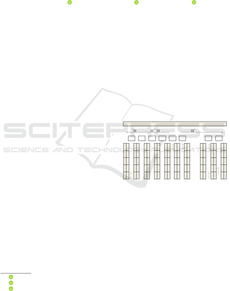
2 THE PROBLEM

The problem input consists of three sets, see Figure 2:

K set of m carts, that form the ﬂeet used to move

parts in the clean room: cart k can carry at most c

lots.

I set of n stations, corresponding to the racks

headed at each machine aisle and used to tem-

porarily host production lots.

R ⊆ I

, set of the service requests that arrive over

time in a given planning horizon T : request r con-

sists of picking up l

lots in station p

and deliver-

ing them to station d

∈ I; also, request r is asso-

ciated with the time t

∈ T from which the associ-

ated lots are available in p

We wish to solve the following problem:

Problem 1. Find cart routes and schedules to deliver

all the lots requested, minimizing the largest comple-

tion time of any request, and also respecting possible

restrictions on cart capacity and operation.

This is a special Dial-a-ride problem, see e.g. (Ho

et al., 2018), with a rectilinear layout of the vehicle

stations. The problem has also the operational con-

straint that a cart cannot drop a lot at a station that

differs from the destination, thus originating a new

request to be fulﬁlled by other carts. Although not

very common in vehicle routing problems, the simple

rack 1 rack 2 rack 3 rack 4 rack 5 rack 6 rack 13 rack 14

………

cart 1 cart 3 cart 2 cart 4

cart 5

request 2

request 1

request 5

request 4

request 3

rack

capacity

WIP levels

cart

capacity

Figure 2: Problem elements.

linear layout has been investigated elsewhere for its

interesting features. (Guan, 1998) considers the prob-

lem of transporting a set of items, each with a spe-

ciﬁc origin and destination, along a path; the Author

observes that minimizing the tour length is NP-hard

if items cannot be dropped at intermediate stations,

while it can be solved in linear time otherwise. (Wang

et al. 2006) propose polynomial-time algorithms to

solve a single-commodity pick-up and delivery prob-

lem on a path using a single cart with unit, or general

ﬁnite, or unlimited capacity. Both studies do not cap-

ture the complexity of our case, where a ﬂeet of carts

is given, each requests involves a separate commodity,

and items cannot be dropped at intermediate stations.

However, in the remainder of the paper we show

how to exploit the rectilinear layout to develop a

math-heuristic algorithm that, cyclically repeated in

the planning horizon, solves Problem 1 in two stages.

3 A MATH-HEURISTIC

Let R

⊆ R be the set of requests that, at some time

t ∈ T , (i) are not yet picked up and (ii) have lots avail-

able at the respective stations. The linear topology

of the central aisle naturally associates every subset

P ⊆ R

with a minimal interval that spans between the

leftmost and rightmost station involved in P, that we

indicate as

a(P) = min

r∈P

, d

} b(P) = max

r∈P

, d

}

For example, consider the requests of Figure 2, as-

suming P = {1, 4, 5}: stations d

= 2, p

= 5, d

= 3

are the leftmost involved in these requests, stations

= 5, d

= 14, p

= 4 are the rightmost; then a(P) =

2, b(P) = 14.

We will in short call any such interval a span.

There are no more spans than pairs of stations in-

volved in R

, i.e. no more than

q(q−1)

= O(q

), where

q = min{n, 2|R

|}: in our case n = 14 implies 91 pos-

sible spans in the worst case. We let S denote the

ICORES 2021 - 10th International Conference on Operations Research and Enterprise Systems

282

set of all those spans, and indicate by w

= b

− a

b(P) − a(P) the width of the s ∈ S associated with

P ⊆ R

. For example, the span s = [2,14] previously

determined has w

= 14 − 2 = 12.

Our heuristic algorithm attempts to solve Problem

1 in two stages that, according to a cluster-ﬁrst route-

second logic, are cyclically repeated at different time

instants t:

1. Assign all the requests of R

to m spans s ∈ S (as

many as the carts in K);

2. Given the set S

∗

of spans obtained from the previ-

ous stage, assign a cart k ∈ K to each s ∈ S

∗

and

schedule its requests.

In stage 1 we cluster requests into spans of con-

venient width — the larger the span the fewer the re-

quests — so that the estimated operation time (travel

+ load/unload) is balanced as far as possible.

In stage 2 we consider simple scheduling poli-

cies where the cart “sweeps” the assigned span from

end to end, changing direction a minimum amount of

times. A relevant feature of those simple policies is

that a solution can easily be reconﬁgured at run time

against possible cart capacity reduction, as well as ur-

gent deliveries or other exceptions. Under the policy

adopted, carts are scheduled with the goal of balanc-

ing operation time.

Details on the two stages are given below.

3.1 Span Selection, Request Allocation

A rough indication of the time a cart would take to

cover a span s is given by

(i) the total volume l

of requests assigned to s: large

correspond to long time spent in load/unload

operations;

(ii) the span width w

: the larger the w

, the longer

will supposedly be the transfer time required to

cover its requests.

While w

only depends on s, the total volume depends

on the requests assigned to s. Let R

denote the set of

requests subsumed by s, i.e., all the r whose pick-up

and delivery stations fall within the ends of s. Then:

∑

r∈R

where x

= 1 if r is assigned to s and 0 otherwise.

Using these variables, plus y

∈ {0, 1} with y

= 1 if

and only if s ∈ S is chosen, we can select the m spans

via the following integer linear program:

min

z∈R

z (1)

z −

− 2u

∑

r∈R

≥ 0 s ∈ S

∑

s∈S

= 1 r ∈ R

≤ y

s ∈ S, r ∈ R

∑

s∈S

≤ m

∑

r∈R

≤ c s ∈ S

, y

∈ {0, 1} s ∈ S, r ∈ R

where S

⊆ S contains all the spans that can accom-

modate request r, v is the average cart speed and u

the nominal load/unload time. Together with the ob-

jective function, the ﬁrst set of inequalities deﬁnes z

as the largest among the estimations of the comple-

tion time required to fulﬁll the requests assigned to a

span. The second set of inequalities ensures that ev-

ery requests is assigned to one span. The third set of

inequalities activates a span when assigned a request.

The remaining inequalities ensure that activated spans

do not exceed available carts, and that cart capacity is

in turn never exceeded.

In its ﬁrst four lines, program (1) has a form close

to an m-centre model, where spans corresponds to fa-

cilities, or centroids, and requests to demand points.

In few words, an m-centre is a set of m points (the

centroids) that minimizes the largest distance between

any demand point and the closest point that belongs

to that set. For a survey on m-centre problems, the

reader is referred to (Calik et al., 2015). Our model

differs from this problem in the distance function, that

includes centroid costs (span lenghts) and, as said, for

the additional knapsack constraints (cart capacities).

Program (1) returns:

• a set S

∗

of m spans;

• a partition {R

: s ∈ S

∗

} of the requests set to be

assigned to carts in the subsequent stage 2;

• a lower bound z

∗

to the minimum time necessary

to schedule all the requests in R

One drawback of program (1) lies in the estima-

tion of transfer time, which is assumed proportional

to the span width w

: this estimate is reasonable if

the cart covers the span in one direction only, but be-

comes very poor if it has to go back and forth. To

obtain a better estimate, we modify program (1) by

distinguishing the requests in R

according to whether

they require a transfer from left to right (forward re-

quests, F

) or from right to left (backward requests,

A Dynamic Dial-a-ride Model for Optimal Vehicle Routing in a Wafer Fab

283

). Precisely

= {r ∈ R

: p

< d

} B

= {r ∈ R

: p

> d

}

We then add 0-1 variables f

, b

, subject to

≤ f

≤ y

r ∈ F

(2)

≤ b

≤ y

r ∈ B

for any s ∈ S. That is, span s is used if a cart uses it

either in forward or in backward direction (or both);

conversely, if not used in forward (backward) direc-

tion, the span cannot be assigned any forward (back-

ward) request. The constraint of model (1) that en-

sures to use ≤ m spans is maintained, but the ﬁrst set

of inequalities, deﬁning the max completion time, is

replaced by

z −

( f

+ b

)

− 2u

∑

r∈R

≥ 0 (3)

for any candidate span s ∈ S. Thus, if the span is as-

signed requests in one direction only, the estimated

travel time is proportional to w

as in model (1), oth-

erwise is proportional to 2w

3.2 Cart Assignment and Schedule

Recall that by our assumption on scheduling (stage

2 of our method), unless an exception occurs, every

cart moves end-to-end in the assigned span minimiz-

ing direction changes. This simple idea can be imple-

mented by different policies, for example:

• Policy 1: the cart picks up parts in the same order

as it ﬁnds them in the travel, and delivers them in

the same order as destinations are encountered.

• Policy 2: the cart ﬁrst operates all the pick-ups in

the order found in the travel; once all parts are col-

lected, the cart delivers them in the order in which

destinations are encountered.

Policy 1 also aims at minimizing the part stack in the

cart, while the goal of Policy 2 is to minimize the

work-in-process at the racks and the time each cart

waits for another: in fact with Policy 2 the pick-up

operations precede every delivery, so we use from

the very beginning the whole cart capacity available

to free racks as far as possible. The best scheduling

method adopted in our experiments follows Policy 1

and works as described next.

In a dynamic context with requests arriving over

time, cart k is in general available from some time

≥ t on, as it is supposed to conclude the deliveries

assigned in the previous time lap. At that time, the

cart will have a particular position ξ

in the aisle and

a particular residual capacity ¯c

. For any s ∈ S

∗

, let

contain the carts whose residual capacity is suf-

ﬁcient to accommodate all the pick-ups in s. Sup-

pose then that span s is assigned to cart k ∈ K

. To

describe the scheduling algorithm implemented for k,

we partition again R

into forward and backward re-

quests F

, B

as in §3.1. If F

is non-empty, let p

) denote the leftmost (rightmost) pick-up (drop)

station among its requests. Similarly, for non-empty

, let p

) denote the rightmost (leftmost) pick-up

(drop) station among its request. For example, with

the requests shown in Figure 2 one has p

= 1, d

14, p

= 13, d

= 2.

Assume both F

and B

non-empty. Then

• if ξ

< a

(that is, the cart starting point lies to the

left of s), k will ﬁrst fulﬁll forward requests, then

backward ones;

• if ξ

> b

, k will ﬁrst fulﬁll backward requests,

then forward ones.

If instead a

≤ ξ

≤ b

, the schedule is constructed

distinguishing three cases

i) ξ

< d

: the cart ﬁrst fulﬁlls the backward re-

quests lying to its left, then changes direction and

fulﬁlls all the forward requests, then ﬁnally gets

back to the remaining backward ones;

ii) ξ

> d

: the cart ﬁrst fulﬁlls the forward requests

lying to its right, then changes direction and ful-

ﬁlls all the backward requests, then ﬁnally gets

back to the remaining forward ones;

iii) d

≤ ξ

≤ d

: we try both the above schedules

and select for the cart the shortest one.

Finally, if F

0, then k has only to fulﬁll back-

ward requests, so it ﬁrst moves to p

and then pro-

ceeds to fulﬁll all requests. A similar schedule with

ﬁrst pick-up in p

is constructed if B

Once, via the rules described above, we have col-

lected the scheduling times τ

for each s ∈ S

∗

and

k ∈ K

, we match carts and spans (and therefore carts

and schedules) once for all, seeking to minimize the

largest completion time C

max

of all the requested ser-

vices. This corresponds to solve a bottleneck match-

ing problem (Garﬁnkel, 1971), (Burkard and Derigs,

1980): unlike ordinary matching, where the weight of

a matching is the sum of the arc weights it consists

of, a matching is here weighted by the largest of its

arc weights. In our case, the problem is deﬁned on

a bipartite graph with node sets K, S

∗

, and arcs (k, s)

deﬁned for every s ∈ S

∗

, k ∈ K

and weighted by τ

An optimal solution to this problem can be found in

O(m

) time (Pundir et al., 2015).

ICORES 2021 - 10th International Conference on Operations Research and Enterprise Systems

284

4 RESULTS

LFoundry provided us with very large and detailed

data samples on clean room operation. Each sample

describes a work shift of over 6 hours, and is formed

by a series of snapshots (one per minute) of request

status. Besides other information, a snapshot gives

the requests pending, those in process and newly ar-

rived ones, all recorded according to the actual prac-

tice of cart routing and scheduling.

On average, 55.7% of the requests are short-

distance, that is, cover < 6 stations in the aisle, and

only 1.8% are long-distance, that is, range over all the

14 stations. More features are given in Table 1 for the

ﬁve samples used in the numerical experience.

Table 1: Sample work shift features.

# requests per snapshot requests

sample snapshots min max avg σ per sample

1 374 38 96 91 0,2 3.110

2 351 32 95 86 0,6 3.076

3 343 41 96 80 0,7 2.984

4 342 45 94 86 0,5 2.902

5 347 54 95 82 0,8 2.943

total 1.757 15.015

From the data available, we deducted average cart

speeds (1.2 m/s) and load/unload times (15 s); then

we tested our approach and compared it to the cur-

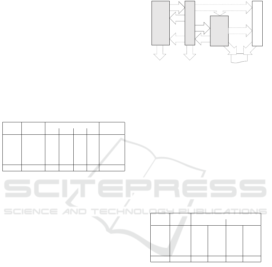
rent practice. The experience was carried out with the

following procedure, see also the scheme in Figure 3:

1. Initialize. Construct the list L of all the requests

in a sample, each with the time of its arrival. Let

t = 0 and let R

contain the requests of the ﬁrst

snapshot.

2. Cycle. Run the algorithm of §3 on the requests

of R

, let C

max

and C

min

be the time length of the

longest and the shortest route of a cart. Take note

of the status (positions ξ

and minimum ready

time t

) of all the carts at t +C

max

3. Update and Repeat. Set t := t +C

min

, create R

including in it all the requests of L that arrived

within [t −C

min

,t]. Taking into account cart status,

go back to step 2 and repeat until all the requests

in L have been fulﬁlled.

We took note of the time t required to complete

all the deliveries in L and compared it to the actual

practice.

The algorithm was encoded in Python 3.7.6. and

run on an Intel core 7,1.8-1.99 GHz processor, 16 GB

RAM, operation system Windows 10 Pro 64-bit ver-

sion 2004. In integer linear programming problems

(1)-(3), the number of variables ranges from a mini-

mum of 2.667 to a maximum of 6.767, that of con-

comparison

quality

indicators

quality

indicators

quality

indicators

quality

indicators

service requests with ready times lots out

lots in

lots out

lots

availability

manufacturing sub-system

transportation

sub-system

storage sub-system (racks)

dial-a-ride model

fleet, speed, l/ul time

Figure 3: Scheme of computational experience: plant

sub-systems (grey blocks), software components (white

blocks), physical ﬂows (solid arrows), main information

ﬂows (dashed arrows).

straints from 2.669 to 6.333. The MIP solver adopted

is Gurobi 9.0.2 with default settings using 8 threads.

All problems were solved to proven optimality.

The ﬁnal outcome is reported in Table 2. All in all,

we processed 15.015 requests for a total work time of

1.757 minutes, see column 2. The result of a numeri-

cal test based on model (1) is reported in columns 3-4,

another test with the model updated by (2), (3) gives

the values in columns 5-6. The former (the latter) test

results in a rough 9% (30%) improvement over ac-

tual practice, amounting in absolute terms to over two

hours and ½ (eight hours and ¾) potentially saved in

ﬁve work shifts.

Table 2: Algorithm performance. Minutes to complete op-

eration, actual duration vs. tests with model (1) and update

(2, 3), and percentage reductions.

sample actual improvement (test)

id. duration model (1) update (2, 3)

1 374 344 8,1% 252 32,7%

2 351 318 9,3% 254 27,5%

3 343 308 10,3% 248 27,7%

4 342 318 7,0% 246 28,1%

5 347 312 10,2% 231 33,5%

total 1.757 1.599 9,0% 1.231 29,9%

The second test gives deﬁnitely better results at

a price, however, of larger CPU times. In fact, ev-

ery cycle (step 2 of the above procedure) took in this

case about 46,4 seconds CPU time on average, rang-

ing from a minimum of 4,9 to a maximum of 147,8

seconds. CPU times of the ﬁrst test were quite shorter:

3,6 seconds on average with a minimum of 1,4 sec-

onds and a maximum of 6,9 seconds.

We also tested our optimization method under Pol-

icy 2 of §3.2. Over all samples, this scheduling policy

returned a completion time of 1.477 minutes, that is

246 minutes (about 20%) worse than Policy 1 but still

280 minutes (16%) better than actual operation.

Besides makespan, it is interesting to observe how

cart workloads are distributed with the proposed ap-

proaches. Table 3 gives, per sample, the mileage

A Dynamic Dial-a-ride Model for Optimal Vehicle Routing in a Wafer Fab

285

covered by the carts. Also under this respect Pol-

icy 1 gives the best result, returning an average cart

mileage 15,7% shorter than that attained by Policy 2

(last row of Table 3). As for route length distribution,

the largest cart mileage with Policy 1 is from 11,6 to

12,9 km shorter than with Policy 2. In absolute terms,

Policy 1 also improves the mileage unbalance of Pol-

icy 2 of amounts ranging between 15,4% and 16,8%.

However, the relative unbalance

longest route − shortest route

longest route

is quite large with both policies, from 48.0% to 51.6%

(51.2% with Policy 2). To correctly read this informa-

tion one has however to consider that program (1)-(3)

tends to assign less lots to longer routes, so as to com-

pensate travel and load/unload time.

Table 3: Mileage balance. Kilometres per cart to complete

operation: average, maximum and unbalance (diff.) per

sample and scheduling policy.

cart mileage (km)

sample id. Policy 1 Policy 2

avg. max diff. avg. max diff.

1 41.4 63.9 31.5 49,5 76.7 37.8

2 42.6 64.2 30.8 50.6 77.1 37.0

3 39.3 62.8 31.7 46.2 75.4 38.0

4 39.6 62.1 31.2 46.5 74.5 37.4

5 38.5 63.8 31.5 48.9 76.6 37.5

tot. avg. 41.2 48.9

Finally, a simple test of the robustness of the

method against parameter variation was done with a

new run of all samples, randomly choosing cart speed

and load/unload time uniformly picked in 1, 2 ± 0, 1

m/s and 15±2 s. With both Policy 1 and 2, this exper-

iment returned a total completion time substantially

close to the values found with constant parameters.

5 CONCLUSIONS

We tackled a challenging vehicle routing problem

arising in the wafer fab of LFoundry, Italy. The prob-

lem has the form of dial-a-ride on a rectilinear topol-

ogy. We developed a math-heuristic that decomposes

the problem into a routing and a scheduling part.

Routes are obtained by solving an integer linear pro-

gram, then are assigned to vehicles by solving a bot-

tleneck matching problem; carts schedules are found

by a simple heuristic method.

The output of the method developed was used in

a large scale numerical test, from which we got clear

indications of possible improvement of plant opera-

tion. The improvement becomes more sensible if a

more accurate estimate of scheduling time is used in

the routing: this entails a trade-off between CPU time

and solution quality although, in general, the method

is very efﬁcient in computational terms and compliant

with on-line operation. To address the rare cases of

non-compliancy, one should accelerate the resolution

of program (1)-(3), which largely dominates the to-

tal solution time. Future research could then consider

to exploit and strengthen, if possible, the highlighted

m-centre structure of the model.

Further improvements of solution quality could be

obtained by reﬁning individual cart scheduling, also

considering different policies. Prior to algorithm im-

plementation in the plant, additional effort should ﬁ-

nally be devoted to construct a simulation model of

the manufacturing sub-system to observe the effect

of an optimized transportation sub-system on the pro-

cess of request generation.

ACKNOWLEDGEMENT

The authors gratefully acknowledge the supportive

cooperation of the team at LFoundry: Mariagrazia

Colotti, Sergio D’Alberto, Fabio Di Vito, Vincenzo

Greco, Massimo Ianni and Raffaele Porzio.

REFERENCES

Burkard, R. and Derigs, U. (1980). The bottleneck match-

ing problem. In Assignment and Matching Problems:

Solution Methods with FORTRAN-Programs, Lecture

Notes in Economics and Mathematical Systems, 184:

60–71. Springer, Berlin-Heidelberg.

Calik, H., Labb

e, M., and Yaman, H. (2015). p-Center

Problems. In: Laporte G., Nickel S., Saldanha da

Gama F. (eds) Location Science, Springer, Cham.

https://doi.org/10.1007/978-3-319-13111-5 4

Garﬁnkel, R. (1971). An improved algorithm for the bot-

tleneck assignment problem. Operations Research,

19(7): 1747–1751.

Guan, D.J. (1998). Routing a vehicle of capacity greater

than one. Discrete Applied Mathematics, 81: 41–57

Ho, S., Szeto, W., Huo, Y., Leung, J., Petering, M., and Tou,

T. (2018). A survey of dial-a-ride problems: Litera-

ture review and recent developments. Transportation

Research B, 111: 395–421.

Pundir, P., Porwal, S., and Singh, B. (2015). A new algo-

rithm for solving linear bottleneck assignment prob-

lem. Journal of Institute of Science and Technology,

20(2): 101–102.

Wang, F., Lim, A., and Xu, Z. (2006). The one-commodity

pickup and delivery travelling salesman problem on a

path or a tree. Networks, 48(1): 24–35

ICORES 2021 - 10th International Conference on Operations Research and Enterprise Systems

286