Mixed Deep Reinforcement Learning-behavior Tree for Intelligent
Agents Design
Lei Li
a
, Lei Wang, Yuanzhi Li
b
and Jie Sheng
Department of Automation, University of Science and Technology of China, Hefei 230027, Anhui, China
Keywords:
Reinforcement Learning, Behavior Tree, Intelligent Agents, Option Framework, Unity 3D.
Abstract:
Intelligent agent design has increasingly enjoyed the great advancements in real-world applications but most
agents are also required to possess the capacities of learning and adapt to complicated environments. In this
work, we investigate a general and extendable model of mixed behavior tree (MDRL-BT) upon the option
framework where the hierarchical architecture simultaneously involves different deep reinforcement learning
nodes and normal BT nodes. The emphasis of this improved model lies in the combination of neural net-
work learning and restrictive behavior framework without conflicts. Moreover, the collaborative nature of two
aspects can bring the benefits of expected intelligence, scalable behaviors and flexible strategies for agents.
Afterwards, we enable the execution of the model and search for the general construction pattern by focusing
on popular deep RL algorithms, PPO and SAC. Experimental performances in both Unity 2D and 3D environ-
ments demonstrate the feasibility and practicality of MDRL-BT by comparison with the-state-of-art models.
Furthermore, we embed the curiosity mechanism into the MDRL-BT to facilitate the extensions.
1 INTRODUCTION
Designing an intelligent agent confronted with com-
plex tasks in diverse environments is generally known
as an intractable challenge. A universally accepted
definition of intelligent agents in (Wooldridge and
Jennings, 1995) indicates that the agent can operate
automatically, perceive environments reactively and
exhibit goal-settled acts initiatively, which demands
for the ability of observing, learning and behaving.
The techniques of employing such intelligent agents
have profound impacts on a wide range of appli-
cations including computer games, scenario simula-
tions, robot locomotion.
Behavior Tree (BT), expressed by (Dromey, 2003)
in the mid2000s, is a well-defined and graphical
framework for modelling AI decision behaviors. As a
replacement of Finite State Machines (FSM) and a fa-
vorable AI approach utilized inherently in games, BT
owns the features of re-usability, readability and mod-
ularity. However, an excellent design of BT needs
enough experience and efforts when the behaviour
representations of agents become increasingly com-
plicated. It’s apparent in the fact that agents with
a
https://orcid.org/0000-0003-3496-9752
b
https://orcid.org/0000-0002-3068-8569
these constrained behaviors have difculty responding
towards dynamically changing environments.
Reinforcement Learning (RL) as one of the
paradigms and methodologies of machine learning
based on Markov Decision Process (MDP) has been
scaled up to a variety of challenging domains, such as
AlphaGo (Silver et al., 2016) and AlphaGo Zero (Sil-
ver et al., 2017), Atari game (Mnih et al., 2013), Sim-
ulated Robotic Locomotion (Lillicrap et al., 2015),
StarCraft (Vinyals et al., 2017), even Vehicle Energy
Management (Liessner et al., 2019). Accordingly,
deep RL gradually emerges with the significant ad-
vance of neural network. Compared with behavior
trees, agents augmented with RL not only can po-
tentially take adaptive strategies, but also learns in-
crementally a complex policy. But deep RL mod-
els are always accompanied with poor sampling ef-
ficiency and limited convergence, lacking a guarantee
of an optimal result. Another cause for the bounded
applicability is the difficulty of designing a reward
function that encourages the desired behaviors all
through training. With respect to hyperparameters,
most methods depend on special settings and easily
get brittle with a small change.
Whether an appropriate model can implement an
intelligent agent with given demands is contingent
upon effective design mechanisms and applicable ex-
Li, L., Wang, L., Li, Y. and Sheng, J.
Mixed Deep Reinforcement Learning-behavior Tree for Intelligent Agents Design.
DOI: 10.5220/0010316901130124
In Proceedings of the 13th International Conference on Agents and Artificial Intelligence (ICAART 2021) - Volume 1, pages 113-124
ISBN: 978-989-758-484-8
Copyright
c
 2021 by SCITEPRESS – Science and Technology Publications, Lda. All rights reserved
113

ecution. As discussed in prior contents, there ex-
ist ubiquitous shortcomings in practicability above.
It’s significant for us to embed the deep RL into
BT and offer a valid model pattern. According to
(de Pontes Pereira and Engel, 2015), a series of sub-
tasks can be abstractly transformed into a reinforce-
ment learning node and in turn BT, profiting from its
hierarchical architecture, can be enhanced reasonably
by absorbing these nodes. In both theoretical and ex-
perimental aspects at last, the model named MDRL-
BT can availably incorporate heteogeneous deep RL
nodes and normal BT nodes to produce a considerable
improvement in intelligent agents design.
2 RELATED WORK
The fundamental theories of BT arouse out of (Mateas
and Stern, 2002; Isla, 2005; Florez-Puga et al., 2009).
(Mateas and Stern, 2002) provided a behavior lan-
guage designed specifically for authoring believable
agents with rich personality as a primitive forerunner.
(Isla, 2005) centering on scalable decision-making
used BT to handle complexity in the Halo2 AI. (Sub-
agyo et al., 2016) enriches behavior tree with emotion
to simulate multi-behavior NPCs in re evacuation.
The deep RL originates from the paper (Mnih
et al., 2013) with the enforcement of CNN network
directly. (Mnih et al., 2015) has stricken a great suc-
cess by developing a deep Q-network (DQN) in this
field. (Schulman et al., 2015) proposes Trust Region
Policy Optimization (TRPO) in policy optimization.
On the basis of TRPO, Proximal Policy Optimization
(PPO) (Schulman et al., 2017) takes the minibatch up-
date and optimizes a surrogate objective function with
stochastic gradient ascent. Soft actor-critic (SAC) are
proposed by Haarnoja (Haarnoja et al., 2018) to max-
imize expected reward and entropy in Actor-Critic
(AC).
The concept of integrating RL into BT has been
put forward to alleviate the endeavors of manual pro-
gramming in some research. (Zhang et al., 2017)
combines BT with MAXQ to induce constrained and
adaptive behavior generation. (Dey and Child, 2013)
presents Q-learning behaviour trees (QL-BT). In the
(de Pontes Pereira and Engel, 2015), a formal den-
ition of learning nodes is applicable to address the
problem of learning capabilities in constrained agents.
Yanchang Fu in (Fu et al., 2016) carries out simu-
lation experiments including 3 opponent agents with
RL-BT. In (Kartasev, 2019) there are detailed descrip-
tions of Hierarchical reinforcement learning and Semi
Markov Decision Processes in BT.
Compared with the relevant works, the contribu-
tions of this paper is intended to contain the follow-
ing aspects: firstly, we demonstrate a general model
MDRL-BT combined flexibly with different deep op-
tions and a simple training procedure to design an in-
telligent agent. Besides, we investigate potential traits
of MDRL-BT for an effective training model. The la-
tent variable generative models and primitive process
of learning can be strengthened with mixed deep RL
algorithms including PPO and SAC by comparative
experiments. Furthermore, we set up experiments on
Unity 3D environment for high quality physics sim-
ulations and revise a simple and unified reward func-
tion about scores and time. Finally, the MDRL-BT
model with curiosity is implemented practically in an
empirical 2D application.
The remainder of this paper is structured in the
following: The introduction of intelligent agents and
corresponding research are presented firstly. After-
wards, the theories of BT and RL and analysis of
MDRL-BT architecture are introduced in detail. In
the model section, we outline the framework based
on options and bring the RL nodes into BT. At the
same time, we facilitate the execution of the model.
In the experiments, we build up some experiments
to search for better performance and draw some con-
clusions from the results. Finally, we summarize the
work and look forward to the future research direc-
tion.
3 PRELIMINARIES
Formally speaking, a behaviour tree is composed of
some nodes and directed edges where internal nodes
called composite nodes and leaf nodes known as ac-
tion nodes are connected by edges.
Each node is classified by the execution strategy
in the following. Sequence, analogies to logical-and
operation, returns Failure once one of the children
fails, otherwise Success. Note that Fallback nodes,
equivalent to logical-or, are appropriate for executing
the first success nodes. Condition nodes represent a
proposition check and instantly return Success if the
condition holds or Failure if not yet. All Action nodes
having specific codes return Success if the action cor-
rectly completes, Failure if it is impossible to con-
tinue and Running when the process is ongoing.
The execution of BT operates with a tick gener-
ated by a root node at a given frequency, which prop-
agates in depth first. When receiving the signal, the
node invokes its execution, enables the corresponding
behaviors or traverses the tick to children. Each node
except root completes with the return status of Run-
ning, Success or Failure, which is transferred to the
ICAART 2021 - 13th International Conference on Agents and Artificial Intelligence
114

parent for determining the next routine. Until the root
node terminates, a new tick always comes into being
from root with a cyclical loop.
The key problem of RL aims at maximizing cumu-
lative rewards in the interactions with environments.
At time step t, the agent in a given state s
t
∈ S de-
cides on an action a
t
∈ A with respect to a mapping
relationship called the policy π : S → A, then receives
a reward signal r
t
and reaches a new state s
t+1
∈ S.
In a given environment, S is a complete description
of state space and A often represents the set of all
valid actions. Generally speaking, the entire sequence
of states, actions and reward can be considered as an
infinite-horizon discounted Markov Decision Process
(MDP), defined by the tuple (S, A, p, r). The state
transition probability p demonstrates the probability
density of the next state s
t+1
in the condition of the
current state s
t
∈ S and action a
t
∈ A. To represent
the long-term cumulative reward, the discount fac-
tor γ is considered to avoid the infinite total reward:
R
t
=
∑
T
i=t
γ
i−t
r
i
(s
i
, a
i
).
In Q-learning, to evaluate the expected return of a
policy, a value function is defined: V
π
(s) = E
π
[R
t
|s
t
=
s] and the state-action value function is the expected
return for an action a performed at state s : Q
π
(s, a) =
E
π
[R
t
|s
t
= s, a
t
= a]. From the Bellman equation,
the recursive relationship can be shown: Q
π
(s
t
, a
t
) =
E
π
[r
t+1
+ γQ
π
(s
t+1
, a
t+1
)|s
t
= s, a
t
= a]. In DQN
(Mnih et al., 2015), a deep convolutional neural net-
work is used to approximate the optimal action-value
function as follows:
Q
∗
(s, a) = max
π
E[r
t
+γr
r+t
+...|s
t
= s, a
t
= a, π] (1)
In the policy network (Silver et al., 2014) , log
loss and discount reward are used to update the pol-
icy guide gradient. The policy can be updated as the
equation:
∇
θ
J(µ
θ
) = E
s∼ρ
µ
[∇
θ
µ
θ
(s)∇
a
Q
µ
(s, a)|
a=µ
θ
(s)
] (2)
Mathematically, the advantage function which is
crucially important for policy gradient methods is de-
fined by A
π
(s, a) = Q
π
(s, a) −V
π
(s). Proximal policy
optimization (PPO) (Schulman et al., 2017) breaks
down the return function into the return function by
the old strategy plus other terms with the monotonic
improvement guarantee and gives a definition of the
probability ratio: r
t
(θ) =
π
θ
(a
t
|s
t
)
π
θ
old
(a
t
|s
t
)
and r
t
(θ
old
) = 1.
The main objective of PPO is the following:
L(θ) =
ˆ
E
t
[min(r
t
(θ)
ˆ
A
t
, clip(r
t
(θ), 1 − ε, 1 + ε)
ˆ
A
t
)]
(3)
Soft Actor Critic(SAC) (Haarnoja et al., 2018), an
extended stochastic off-policy optimization approach
based on actor-critic formulation, centers on entropy
regularization to maximize a trade-off between explo-
ration and exploitation with the acceleration of the
learning process. The agent at every time step obtains
an augmented reward proportional to the expected en-
tropy of the policy over ρ
π
with trade-off coefficient
α:
J(π) =
T
∑
t=0
E
(s
t
,a
t
)∼ρ
π
[r(s
t
, a
t
) + αH (π(·|s
t
))] (4)
4 MODEL
The general approach for maintaining the superiority
of RL and BT together is to apply the option frame-
work to BT. On this basis, deep RL algorithms can be
imbedded unaffectedly in the learning nodes to obtain
observation information and make decisions in accor-
dance with the learned policy. In the meantime, the
learning nodes are claimed to keep the feasible and
constrained characteristics of normal nodes. Deriv-
ing from recursive BT, the generated model MDRL-
BT stresses on a relatively simple and efficient real-
ization and implements an optimized execution with
these nodes.
4.1 The Option Framework in BT
The central trait of MDRL-BT focuses on an idea that
a big task can be decomposed into multiple smaller
tasks in BT and several nodes associated with a task
can aggregate into a learning node. Each divided
task reduces the non-linear increase of dimensional-
ity with the size of the observation and action space,
similar to the essence of Hierarchical Reinforcement
Learning (HRL) and Semi Markov Decision Pro-
cesses (SMDP) based on the option framework pro-
posed in (Sutton et al., 1998). In the framework, a
primary option is initialized in a certain state and then
a sub-option is adopted by the learning strategy. After
that, the sub-option proceeds until it terminates and
another option continues like the running process of
BT.
An option is a 3-tuple consisting of three elements
< I , π, β > where : I ⊆ S indicates the initial state of
option, π : S × O → [0, 1](O =
S
s∈S
O
s
) represents the
semi-markov policy which is a probability distribu-
tion function based on state space and option space,
µ : S × O × A → [0, 1] with additional action space
defines the intra-option policy. For each state s, the
available options are represented by O(s). When the
present state s is an element of I , a corresponding op-
tion is successfully initialized. The bellman equation
Mixed Deep Reinforcement Learning-behavior Tree for Intelligent Agents Design
115

for the value of an option o in state s can be expressed:
Q
π
O
(s, o) = Q
µ
O
(s, o) +
∑
s
0
P(s
0
|s, o)
∑
o
0
∈O
s
π(s
0
, o
0
)Q
π
O
(s
0
, o
0
)
(5)
The current option chooses the next option o with
the probability π(s, o) during the execution and then
the state can change to s
0
. Moreover, the definition of
the intra-option value function is:
Q
µ
O
(s, o) =
∑
a
µ(a|s, o)Q
U
(s, o, a) (6)
where Q
U
: S × O × A → R represents the action
value in a state-option pair according to (Bacon et al.,
2017):
Q
U
(s, o, a) = r(s, a) + γ
∑
s
0
P(s
0
|s, a)U(o, s
0
) (7)
β : S → [0, 1] is the termination condition and β(s)
means that state s has the probability β(s) of termi-
nating and exiting the current option. The value of o
upon the arrival of state s
0
with the probability β(s
0
)
of option termination, U(o, s
0
) is written as:
U(o, s
0
) = (1 − β(s
0
))Q
µ
O
(s
0
, o) + β(s
0
)V
O
(s
0
) (8)
In the context of BT, the termination condition β
is bound up with the return status of Failure or Suc-
cess. A new episode starts when an option is acti-
vated by a signal tick for a timestep and ends up with
the termination of option. With regard to Running,
it accounts for the process of an option node with a
consecutive series of uninterrupted ticks in BT. This
would imply that the ticks complete the synchroniza-
tion with RL algorithm. As far as an MDP problem
is concerned, the option collects the actions, rewards
and states stored in trajectories D, which updates the
option-option policy π or intra-option policy µ. In
general, traditional composite and decorator nodes in
BT have a fixed policy for calling their children se-
quentially. In this paper, we remove the limitations for
the utilization of option framework so that the policy
π could rearrange the execution order of children.
4.2 Reinforcement Learning Nodes
Based on the previous theorem (de Pontes Pereira and
Engel, 2015), learning action and composite nodes
are referred to as the extensions of the normal BT
nodes. These learning nodes not only successfully are
equipped with the learning capacities , but also main-
tain the readability and modularity in hierarchical BT
framework. For learning composite nodes, the notion
of learning fallback nodes is defined as follows.
Definition 1. A learning fallback node below at-
tached with children c
1
, c
2
..., c
n
as possible choosing
Figure 1: The transformation from several normal nodes to
a learning node with observations, reward functions, policy
and actions.
sub-options can be modelled as an option with an in-
put set I = S, an output order (c
i
1
, c
i
2
..., c
i
n
), a termi-
nation β = 1 if any Tick(c
i
) ∈ Success or all Tick ∈
Failure and a policy π.
The learning Fallback nodes can query the rele-
vant children every episode in learned priority instead
of the constant order. The corresponding learned pol-
icy π, according to the observations mainly correlated
with the state of the environment, devotes to decid-
ing one of the children and then holding a series of
updates during execution. The learning Sequence re-
sembling learning Fallback just differs in the termi-
nation condition β = 1 if any tick(c
i
) ∈ Failure or all
ticks ∈ Success. The example of learning composite
nodes involving SAC is illustrated in algorithm 1.
Definition 2. A learning action node can be modelled
as an option with an input set I = S, actions a ∈ A
s
, a
termination condition β, and a policy µ.
In most cases, MDRL-BT abstracts a subtree into
a learning action node for potential performance and
Algorithm 1: SAC composite nodes with N children.
Input: an input set I = S , initial state value func-
tion parameters φ, φ and soft Q-function paremeters
ψ, tractable policy θ parameters, count steps k = 0.
Output: Failure, Suceess, or Running
1: state is Failure if Sequence, Success if Fallback
2: if a tick arrives then
3: collect global state s
k
, run policy π
θ
, take ac-
tion a
k
∈ A and get an index order i
1
, i
2
..., i
N
4: for j ← 1 to N do
5: childstatus ← Tick(child(i
j
))
6: if childstatus=Running then
7: return Running
8: else if childstatus=state then
9: goto → line 11
10: state ← ∼state
11: receive reward r
k
, add tuple (s
k
, a
k
, r
k
, s
k+1
) to
trajectories D
k
, update the parameters(i ∈ {1, 2}):
φ ← φ − λ
V
ˆ
∇
φ
J
V
(φ), ψ
i
← ψ
i
− λ
Q
ˆ
∇
ψ
i
J
Q
(ψ
i
)
θ ← θ − λ
π
ˆ
∇
θ
J
π
(θ), φ ← τφ + (1 − τ)φ, k ← k + 1
12: return state
ICAART 2021 - 13th International Conference on Agents and Artificial Intelligence
116

Figure 2: The structure of MDRL-BT contains four categories. The blue option nodes refer to the two kinds of learning nodes
with deep RL algorithms. The blank nodes indicate the normal BT nodes and the green rectangle with imaginary line is not a
tree node but the input of external state of environment or initial design settings.
simplification. In figure 1, the entire BT can be turned
into a learning action node for an enemy attack in
this simple case. In short, the learning action nodes
carry through an MDP to define the evolution of agent
states. The learning action nodes with PPO can be
summarized in algorithm 2.
Algorithm 2: PPO learning action nodes.
Input: an input set I = S, initial policy parameters
θ, value function parameters φ, count steps k = 0.
Output: Failure, Suceess, or Running
1: if a tick arrives then
2: collect local state s
k
, run policy π
θ
old
, take ac-
tion a
k
∈ A, and receive reward r
k
3: if the task goal is finished then
4: return Success
5: else if impossible to finish then
6: return Failure
7: else
8: add (s
k
, a
k
, r
k
, s
k+1
) to the trajectories D
k
,
compute rewards-to-goes
ˆ
R
t
, and compute the ad-
vantage estimates
ˆ
A
t
, based on value function V
φ
k
.
9: Update the policy parameter:
θ = argmax
θ
ˆ
E
t
[min(r
t
(θ)
ˆ
A
t
, clip(r
t
(θ), 1 −ε, 1 +ε)
ˆ
A
t
)]
φ = argmin
φ
ˆ
E
t
[(V
φ
(s
t
) −
ˆ
R
t
)
2
]
10: θ
old
← θ, φ
old
← φ, k ← k + 1
11: return Running
4.3 MDRL-BT Architecture
In this section, we will systematically illustrate the ex-
tended architecture of MDRL-BT and analyze respec-
tively the different functions of every node area. As
stated in figure 2, it is a recursive BT as a whole with a
core option and four types of divided areas, in keeping
with the hierarchies of option framework. It deserves
to be mentioned that every periodic tick represents a
temporal level of timescale signal propagating from
top to down and activates the running courses of trig-
gered nodes. The core option as a representative of
the core logic abstraction from complicated tasks can
also be replaced with normal composite nodes with a
fixed execution setting. The children of core option is
roughly classified on the grounds of types of nodes.
Although the four areas are distinct, every area is di-
rectly connected with the core option and can be inter-
spersed disorderly with every independent individual
of other areas. The parameter N in every area is also
different, ranging from zero to infinity.
The blue option nodes are the learning compos-
ite nodes with discrete outputs. In conjunction with
global state input relative to the local state, this type
of nodes can distill global observations to dispense
the order index of children. As seen in figure 2, the
recursive sub-tree can follow the option node with the
same framework of four areas generation after gener-
ation. So the recusive sub-tree can be large or small
depending on specific tasks and in this perspective the
Mixed Deep Reinforcement Learning-behavior Tree for Intelligent Agents Design
117

MDRL-BT combined with this type of node can be in
possess of flexible structure and have certain general-
ity in applications.
The blue action nodes are the learning action
nodes which collects the local state to improve pol-
icy with continuous or discrete actions. The nodes
with meticulous reward function can facilitate imple-
mentation of subtask and simplify large-scale archi-
tecture. In the presence of several learning action
nodes with the similar action space, reward function
and task goals, it is recommended that a RL brain can
be independent of these nodes and keep parallel con-
nection for reusability and time saving, such as details
in Experiment 1. Accompanying the MDRL-BT with
this blue action nodes in essence extends the BT to
MDRL-BT.
Composite nodes and action nodes are subsumed
together into blank nodes. For the blank option nodes
they can be conventional identified types of Fallback,
Sequence, Parallel, Decorator mentioned above. The
priority setting, p(s) → R mapping the state to pri-
ority value, is the function of the execution order de-
signed initially as the input. The blank nodes of Ac-
tion or Condition with typical commands are com-
mon indivisible units. As the granularity of MDRL-
BT, the executable action nodes can be defined prefer-
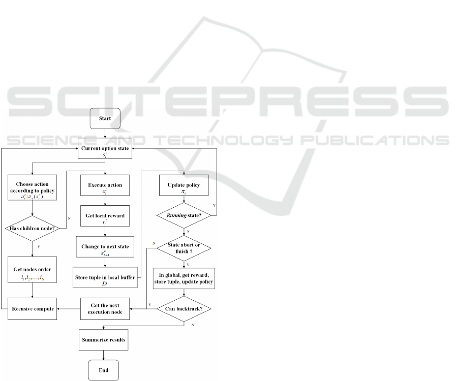
Figure 3: The execution process of MDRL-BT. It is actu-
ally a nested process with inter-option and intra-option pol-
icy distinguished by having children. The traditional nodes
suffer from stationary policies and are ignored selectively.
ably with the demonstrations for solving complicated
problems and improving learning efficiency of the
tree.
A myriad of flexible classical algorithms are in-
corporated concurrently when different blue nodes are
adopted, giving rise to the nature of BT. It’s plausible
that MDRL-BT can reap the advantage of BT and RL
and can vary with practical applications to cater for
designers’ needs. The next part would introduce the
execution process and effective reward function.
4.4 MDRL-BT Execution
There are N learning children of core option with
unfixed execution time interval T
n
, policy π
n
, the
corresponding state S
n
, action space A
n
, reward R
n
(n ∈ [1, N]) and M normal nodes with time interval
T
m
and degree of goal completion G
m
. Uniformly the
core option has T
c
,π
c
,S
c
,A
c
,R
c
. Along with the begin-
ning of MDRL-BT, the core option gathers observa-
tion s
c
∈ S
c
and take an action a
c
∈ A
c
, get the tuple
results of index order (i
1
, i
2
..., i
N
). At the time t, we
can get the following equation.
(i
1
, i
2
..., i
N
)
t
= a
c
t
|π
c
(s
c
t
), a
c
t
∈ A
c
, s
c
t
∈ S
c
, (9)
The execution flow of MDRL-BT can be summa-
rized detailedly in figure 3. Up to now, the tuple
< s
c
t
,a
c
t
,r
c
t
,s
c
t+1
>, where s
c
t+1
is the global state of next
episode, can be stored in its buffer trajectories τ for
experience replay. The subsequent procedure may be
easily adapted to other learning options with a plural-
ity of subspaces because of the recursive inference for
subtree. In the local time interval, the children moti-
vate MDPs, considered explicitly as the sub episode
of the high level.
It’s an assumption that the first k children nodes
has finished with Success status and the i
k+1
node
aborts the next execution. It is derived that the total
time of core option is the sum of first k normal exe-
cution time where ε is the total error of transfroming
time and T
c
corresponds to the amount of the whole
tree execution time.
T
c
=
k
∑
j=1
T
i
j
+ ε (10)
The reactive rewards function needs to reflect the
tendency of goal-achieving in a sense. In the ordi-
nary way, the rewards are tied to the execution time
and degree of task completion, and should be normal-
ized theoretically for training performance. In this pa-
per, the abort status doesn’t exist in scenarios where
the core option can execute the all children nodes
k = M + N. Hereby, the mixture rewards of core op-
ICAART 2021 - 13th International Conference on Agents and Artificial Intelligence
118

tion can be computed in the following.
r
i
t
=
(
f
1
i
(T
i
(t))+ f
2
i
(G
i
(t)) i ∈ normal nodes
f
1
i
(T
i
(t))+ R
i
(t) i ∈ learning nodes
(11)
r
c
t
= Normalize(
M+N
∑
i=1
r
i
t
), r
i
t
∈ R
i
(12)
where f
1
i
is always a piecewise function for reducing
the time error ε and f
2
i
is a mapping function for goal
achievement. The equation is not the only rewards de-
sign but can sometimes be a more reasonable choice
than the others.
Thus far, MDRL-BT has made use of option
framework to ascertain usability in a theoretical man-
ner. This conjugated model with this hierarchical de-
sign for the intelligent agents, compatible with the
structure of BT, mixes nodes together and can over-
come the weakness of the RL and BT. In the model, it
turns out to be that the learning can be undertaken in
tandem by mixed RL nodes and the constrained run-
ning is solely in the charge of BT. MDRL-BT with
the underlying option framework has circumvented
the conflicts between BT and RL and can be easily
altered for different targets. In the next section, we
will do some experiments for comparison and mani-
fest operability.
5 EXPERIMENTS
Several valuable experiments with various complex-
ity are performed in this section to identify the char-
acteristics of MDRL-BT and validate the intelligent
agents. Most experiments are consequently con-
ducted and measured on Unity 3D environments close
(a) experiment 1 2 env. (b) experiment 3 env.
(c) corgi env in global. (d) corgi env in local.
Figure 4: The unity 3D environments (a)(b) of experiments
and the high fidelity makes it possible for agents to bring
evidence towards the application of model. Details and dis-
cussion of experiments are released in the description sec-
tion. Corgi environment (c)(d) with an extendable engine
is a friendly 2D game where agents can finish some simple
tasks.
(a) experiment 1 2 env. (b) experiment 3 env.
Figure 5: The plane environments. Every tagged objects
would be labelled by arrows. Four discrete actions only be
taken by the agent to achieve the taskmove forward, move
backward, turn left, turn right. Furthermore, the agent is
provided by a view fan field composed by a number of ray
sensors as the primary observations which can detect the
corresponding objects. The apparent information of relative
positions, rotations and distances, are added collectively up
to 109 and 1490 observations.
to real-world situations for generality and veracity. In
order to take a deep dive into the traits of MDRL-BT,
the training models are configured with different con-
structions and components as comparison. The Unity
ML-Agents Toolkit (Juliani et al., 2018), accessible to
the wider research, serves as an open-source project
and can be used to train intelligent agents through a
simple-to-use Python API. In (Noblega et al., 2019),
adaptable NPC-agent with PPO has been devised in
Unity ML-Agents Toolkit environments as an enlight-
enment of experimental simulations.
5.1 Description
Inspired by (Sakr and Abdennadher, 2016) in which
rescue and saving simulation involves task plan-
ning and realistic estimations, experiment 1 is es-
tablished by extending simulated fire control scenar-
ios (de Pontes Pereira and Engel, 2015) to a 3D en-
vironment in figure 4(a)(b) for agent training. Ex-
periment 1 and 2 almost take place in an identical
surroundings where independent RL can accomplish
the benchmarks and the proposed MDRL-BT would
combat the challenges of baselines. With regard to
complex relationship in experiment 3, significant ad-
vances in performance are made by MDRL-BT irre-
spective of training and testing. And an agent attached
with MDRL-BT on a 2D game about corgi engine is
heightened by the driven-curiosity learning for a fur-
ther expansion.
The standard of scores acquired by agent for eval-
uation is measured by the degree of target completion
and the frequency of collisions with the walls. Simul-
taneously, the total time of each episode is collected
separately for the estimation of completion speed.
Mixed Deep Reinforcement Learning-behavior Tree for Intelligent Agents Design
119

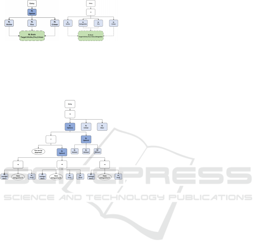
(a) model in exp1. (b) model in exp2.
Figure 6: The models of two experiments. The solid lines
are ticks flowing between nodes and the imaginary lines
proceed with an interaction between blue nodes and green
brain. The RL option in dark blue is a learning compos-
ite node in all experiments and the RL nodes in watery blue
are learning action nodes aiming at sub-tasks like saving the
victim. Other blank nodes are nothing but normal nodes.
Figure 7: The mixed model described is composed of 12
watery blue PPO learning action nodes with a shared brain,
3 dark blue SAC composite learning options with different
configurations and another 9 blank normal BT nodes.
In order to assess the results equally and exactly,
the mean values of every experiment upon thirty-two
thousand times are calculated. Consistent with the
general learning process, incremental steps and re-
wards of feedback during the training are kept track
of to understand the convergence.
Experiment 1. As enumerated in plane figure
5(a), there are four types of objects characterized by
victim, fire, criminal and agent. The task refers to it
that the agent is bound to save victim, extinguish the
fire and catch criminal as soon as possible. For ev-
ery episode, the agent is commanded to accomplish
the task spontaneously but the four objects are ini-
tially placed or reset in a random pattern to eliminate
the training contingency. This scenario is surrounded
markedly by high walls in figure 5(a)(b) to prohibit
stepping outside. Afterwards, the ground without
friction appears so smooth that the agent with man-
ual control is indeed difficult to manipulate in discrete
action spaces.
As aforementioned, the state-of-arts of off-policy
SAC (labelled as SAC) and on-policy PPO (PPO)
are implemented separately to establish a test base-
line and opsive behavior designer is integrated by
Unity NavMeshAgent to build a normal BT with-
out the need of training (BT). To employ the ver-
satile framework of MDRL-BT appropriately, learn-
ing action nodes at first are assigned as children of a
sequence node in BT which is identical to the con-
struction in figure 6(a) except option nodes. The se-
quence node as a core attempts to control the main
process and the action nodes with SAC (BT
sac
) and
PPO (BT
ppo
) opt to act from the learned strategy. In
the cost of more observations and changing inputs, the
different action nodes can be connected with a shared
RL brain to speed up training in terms of the similar
strategy.
Undoubtedly, the sequence node above with a
constrained querying pattern may lead to a sub-
optimal consequence on account of hardly inevitable
order, which is also the universal self-imposed restric-
tions in general BT. We replace the sequence node
by RL option node as the figure 6(a) shows, which
is indicative of the breakthrough point of the limited
structure. The core option node serves as a global
decision maker to explore a better consequence, cal-
culating specific target value and scheduling the ex-
pected queries with learning policy. Accordingly,
there are two promising alternative options with PPO
(Option
ppo
) and SAC (Option
sac
) for further training.
For removing the impacts of learning action nodes,
PPO action nodes aren’t modified in the two models.
Taking the time of training into consideration, we also
use a previously trained PPO action node in the start
to apply the option with SAC(Option
pre
).
Experiment 2. On the foundation of the preced-
ing subject in experiment 1, an extinguisher marked
green is placed as a vital part of the environment and
the sequential order of three independent tasks is de-
manded to confirm the positive features of BT in ex-
periment 2. The agent certainly acquires an extin-
guisher intended for addressing the fire issue ahead
of time, otherwise approaching the fire within certain
distances leads to a punishment of reward and score.
The model described in figure 6(b) is dominated by a
sequence node in this restrictive and flexible circum-
stance. For comparative analysis, the training holds
fixed steps of 3 ∗ 10
7
.
Experiment 3. An increasingly complicated re-
quest arises that the agent struggles to undertake three
victims saving and put out two types of fire previ-
ously, then catch a criminal and enter the door to
restart a period lastly in figure 5(b). Meanwhile,
three extinguishers with corresponding tags are as-
sociated with the assumption that extinguisher1 only
deals with fire1, extinguisher2 only for fire2 but extin-
ICAART 2021 - 13th International Conference on Agents and Artificial Intelligence
120

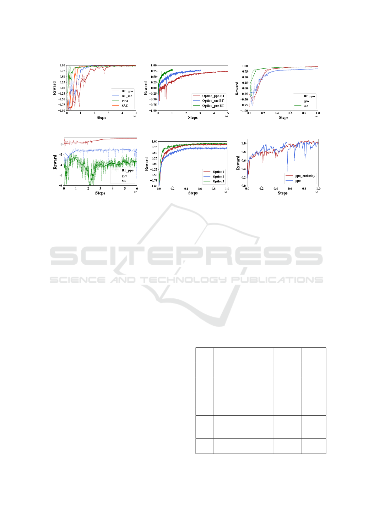
(a) exp1 training. (b) exp1 training. (c) exp2 training.
(d) exp3 training. (e) exp3 training. (f) corgi training.
Figure 8: The training curve of experiments. Because learning composite options are different from learning action nodes
in training frequency. So experiment 1 and experiment 3 would have two graphs. Experiment 2 and corigi without learning
composite nodes only have one graph. Every curve with corresponding tag means an algorithm with the same conditions in a
graph.
guisher3 for fire1 and fire2 both. That’s the same case
that every object is generated arbitrarily in any cor-
ner of the environment and more walls are added to
hamper the movement of the agent. What’s more, the
victims, extinguishers and fire may be randomly ab-
sent at the outset of every episode. This highlights the
dynamically changing of the environment and reaches
the number of 2
8
kinds of different situations totally.
In addition, the active criminal is moving all the time
with a slow velocity and will stay away from the agent
within a certain distance in the face of agent.
5.2 Results and Analysis
In this section, the performances for the trials are sub-
jected to contrastive analysis. The examinations are
carried out to corroborate the benefit of mixed com-
ponents.
PPO vs SAC. Figure 8(a) indicates that indepen-
dent PPO and SAC can rapidly converge. Although
the reward of SAC with the preponderance of sample-
efficient learning can get close to one in a short time
and in contrast it takes a long time for PPO to ar-
rive, it is apparent in table 1 and figure 9 that in the
perspective of scores and time the PPO outperforms
readily SAC due to the influence of the sensitive hy-
perparameters tuning and frequent policy updates of
SAC in discrete action space. Therefore, it is hy-
pothesized that PPO is more applicable to the fre-
quent movement manipulation of agents than SAC
which is the same difference between PPO(BT
ppo
)
and SAC(BT
sac
). PPO(BT
ppo
) appears more stable
and behaves as well as the independent RL on the ta-
ble 1 but it takes more steps to converge. Adopting
PPO nodes can yield the better objective of scores and
time.
MDRL-BT vs RL. According to the quantitative
analysis of training steps in experiment 2, the frame-
Table 1: Evaluation statistics. Exp is about experiment type.
S and T respectively show scores and time. Mean means an
average value. The full score reaches 100 and the unit of T
is seconds.
Exp Model Mean S Mean T Train
1
BT 92.4365 13.2821 -
PPO 96.5761 9.0265 10
7
SAC 95.4983 13.1198 10
7
BT
ppo
96.5513 9.5955 10
7
BT
sac
96.1467 11.2166 10
7
Option
ppo
97.4605 8.8977 5 ∗ 10
6
Option
sac
97.7533 8.5394 3 ∗ 10
6
Option
pre
97.7208 8.2931 1 ∗ 10
6
2
PPO 71.2845 12.2972 3 ∗ 10
7
SAC 84.8081 17.5410 3 ∗ 10
7
BT
ppo
94.2582 12.3749 3 ∗ 10
7
3
other - - 1 ∗ 10
8
mixed 90.2595 19.5666 1 ∗ 10
8
Mixed Deep Reinforcement Learning-behavior Tree for Intelligent Agents Design
121

(a) exp1 score. (b) exp1 time.
(c) exp2 score. (d) exp2 time.
Figure 9: The distribution of 32000 tests suggests the average value and the standard deviation. The corresponding conclusion
can be drawn clearly on the grounds of the results. In experiment 3, only the mixed model can get a positive score in a limited
time. So the result isn’t shown.
work for modeling constrained yet adaptive agents re-
veals the character of BT and surpasses the behavior
of PPO and SAC quite a few. The sequential strategy
time-consuming for the independent RL algorithms is
exhibited favorably by MDRL-BT for simplification
and efficiency.
Option Nodes. Table 1 especially shows that
all models with learning core option and PPO ac-
tion nodes can outperform the other methods and
present an optima. Respectively, Option
sac
with less
training steps but thoroughly performs better than
Option
ppo
from figure 8(b) and table 1, because SAC
is particularly appropriate for low frequency updates
and its sample efficiency consequently exceeds PPO.
Option
pre
with pre-trained action nodes can almost
keep in line with Option
sac
in scores with the less
steps. It is indicated that Option
pre
can be a supe-
rior choice in complicated models for the reduction of
training steps. To sum up, learning action nodes with
PPO deals with complex environmental dynamics and
option nodes with SAC quickly handle planning and
scheduling in the construction of MDRL-BT.
MDRL-BT vs Others. The behavior of wall
touching or breaking rules with a reduction of scores
and rewards in experiment 3 makes the scenario no-
ticeably troublesome and the agent must be in posses-
sion of some intelligence to manage and conduct its
behavior across the environment. In figure 8(d), the
independent PPO and SAC which beforehand fall into
a local dilemma hardly proceed with training and a
simple model of BT
ppo
is incapable of achieving good
performance due to the dynamic rewards and the pun-
ishment of far too much walls touching. Nevertheless,
the MDRL-BT with the model in figure 7 successfully
addresses the issues as table 1 and figure8 (e) shows.
2D. On the basis of 3D experiment, we explore
the 2D game environment in figure 4(c)(d) built by
corgi engine to verify the other features of MDRL-
BT model. The corgi agent with BT
ppo
is required
to collect the coins scattered all over the corners in a
limited time. What’s more, curiosity is employed in
the MDRL-BT and in figure 8(f) both models can be
trained well enough but curiosity (Burda et al., 2018)
can get a little better result.
6 CONCLUSIONS
This paper has researched a mixed model for invent-
ing an intelligent agent. We do some surveys on con-
textual backgrounds and related studies to explore the
promotion of agent designs. Enough efforts about
the combination of deep RL and BT have been made
by digging deep into the theoretical basis and ex-
isting correlations. As a specialization of option-
framework, MDRL-BT architecture is refined on the
strength of deep learning nodes and BT construction.
We accomplish the execution synchronization of RL
and BT and define an appropriate rewards function to
prescribe the desired decisions. Several virtual simu-
lations are implemented on Unity 2D and 3D environ-
ments to employ semantics and structure of MDRL-
BT. The mixed model also varies slightly with the
complexity for displaying the special attributes.
The insights gained from results may be of assis-
tance to intelligent agents. MDRL-BT, reflecting the
integrated advantage in the theorem, empirically out-
weights the BT and RL and can be successfully ap-
plied to 2D and 3D environments. When especially
faced with complicated affairs or sequential tasks, the
ICAART 2021 - 13th International Conference on Agents and Artificial Intelligence
122

MDRL-BT keeps the mind of hierarchies by decom-
posing a main issue into several simple questions to
provide a rational alternative solution. As evident
from the result, MDRL-BT doesn’t need elaborate re-
ward design to guarantee the training convergence rel-
ative to general RL algorithms. In the design of mixed
models, its a better choice to use PPO action nodes
with a shared brain and SAC composite nodes, even
pre-train nodes. So as to a real available application,
general RL algorithms or normal BT can be used for
simple tasks and by the way, MDRL-BT can be a can-
didate for complex problems.
MDRL-BT has a certain extensibility because of
recusive BT framework and RL foundations. Some-
times further exploration for extending MDRL-BT by
importing other mechanisms such as curiosity in the
sparse reward distribution can be an exciting avenue.
However, there will be enormous work to finish from
the unconspicuous consequence. In the future work,
the correlative theory and applicable scene about the
additional algorithms can be investigated for better
performance.
REFERENCES
Bacon, P.-L., Harb, J., and Precup, D. (2017). The option-
critic architecture. In Thirty-First AAAI Conference
on Artificial Intelligence.
Burda, Y., Edwards, H., Pathak, D., Storkey, A., Dar-
rell, T., and Efros, A. A. (2018). Large-scale
study of curiosity-driven learning. arXiv preprint
arXiv:1808.04355.
de Pontes Pereira, R. and Engel, P. M. (2015). A framework
for constrained and adaptive behavior-based agents.
arXiv preprint arXiv:1506.02312.
Dey, R. and Child, C. (2013). Ql-bt: Enhancing behaviour
tree design and implementation with q-learning. In
2013 IEEE Conference on Computational Inteligence
in Games (CIG), pages 1–8.
Dromey, R. G. (2003). From requirements to design: for-
malizing the key steps. In International Conference
on Software Engineering and Formal Methods.
Florez-Puga, G., Gomez-Martin, M., Gomez-Martin, P.,
Diaz-Agudo, B., and Gonzalez-Calero, P. (2009).
Query-enabled behavior trees. IEEE Transactions
on Computational Intelligence and AI in Games,
1(4):298–308.
Fu, Y., Qin, L., and Yin, Q. (2016). A reinforcement learn-
ing behavior tree framework for game ai. In 2016 In-
ternational Conference on Economics, Social Science,
Arts, Education and Management Engineering, pages
573–579.
Haarnoja, T., Zhou, A., Abbeel, P., and Levine, S. (2018).
Soft actor-critic: Off-policy maximum entropy deep
reinforcement learning with a stochastic actor. In
ICLR 2018 : International Conference on Learning
Representations 2018.
Isla, D. (2005). Gdc 2005 proceeding: Handling complexity
in the halo 2 ai. Retrieved October, 21:2009.
Juliani, A., Berges, V., Vckay, E., Gao, Y., Henry, H., Mat-
tar, M., and Lange, D. (2018). Unity: A general plat-
form for intelligent agents. arXiv:1809.02627.
Kartasev, M. (2019). Integrating reinforcement learning
into behavior trees by hierarchical composition.
Liessner, R., Schmitt, J., Dietermann, A., and Bker, B.
(2019). Hyperparameter optimization for deep re-
inforcement learning in vehicle energy management.
In Proceedings of the 11th International Conference
on Agents and Artificial Intelligence - Volume 2:
ICAART,, pages 134–144. INSTICC, SciTePress.
Lillicrap, T. P., Hunt, J. J., Pritzel, A., Heess, N., Erez, T.,
Tassa, Y., Silver, D., and Wierstra, D. (2015). Contin-
uous control with deep reinforcement learning. arXiv
preprint arXiv:1509.02971.
Mateas, M. and Stern, A. (2002). A behavior language for
story-based believable agents. IEEE Intelligent Sys-
tems, 17(4):39–47.
Mnih, V., Kavukcuoglu, K., Silver, D., Graves, A.,
Antonoglou, I., Wierstra, D., and Riedmiller, M. A.
(2013). Playing atari with deep reinforcement learn-
ing. arXiv preprint arXiv:1312.5602.
Mnih, V., Kavukcuoglu, K., Silver, D., Rusu, A. A., Ve-
ness, J., Bellemare, M. G., Graves, A., Riedmiller,
M., Fidjeland, A. K., Ostrovski, G., Petersen, S.,
Beattie, C., Sadik, A., Antonoglou, I., King, H., Ku-
maran, D., Wierstra, D., Legg, S., and Hassabis, D.
(2015). Human-level control through deep reinforce-
ment learning. Nature, 518(7540):529–533.
Noblega, A., Paes, A., and Clua, E. (2019). Towards adap-
tive deep reinforcement game balancing. In Proceed-
ings of the 11th International Conference on Agents
and Artificial Intelligence - Volume 2: ICAART,, pages
693–700. INSTICC, SciTePress.
Sakr, F. and Abdennadher, S. (2016). Harnessing super-
vised learning techniques for the task planning of am-
bulance rescue agents. In Proceedings of the 8th In-
ternational Conference on Agents and Artificial In-
telligence - Volume 1: ICAART,, pages 157–164. IN-
STICC, SciTePress.
Schulman, J., Levine, S., Moritz, P., Jordan, M. I., and
Abbeel, P. (2015). Trust region policy optimization.
arXiv preprint arXiv:1502.05477.
Schulman, J., Wolski, F., Dhariwal, P., Radford, A., and
Klimov, O. (2017). Proximal policy optimization al-
gorithms. arXiv preprint arXiv:1707.06347.
Silver, D., Huang, A., Maddison, C. J., Guez, A., Sifre, L.,
Den Driessche, G. V., Schrittwieser, J., Antonoglou,
I., Panneershelvam, V., Lanctot, M., et al. (2016).
Mastering the game of go with deep neural networks
and tree search. Nature, 529(7587):484–489.
Silver, D., Lever, G., Heess, N., Degris, T., Wierstra, D.,
and Riedmiller, M. (2014). Deterministic policy gra-
dient algorithms. In Proceedings of the 31st In-
ternational Conference on International Conference
Mixed Deep Reinforcement Learning-behavior Tree for Intelligent Agents Design
123

on Machine Learning - Volume 32, ICML’14, page
I387I395. JMLR.org.
Silver, D., Schrittwieser, J., Simonyan, K., Antonoglou, I.,
Huang, A., Guez, A., Hubert, T., Baker, L., Lai, M.,
Bolton, A., et al. (2017). Mastering the game of go
without human knowledge. Nature, 550(7676):354–
359.
Subagyo, W. P., Nugroho, S. M. S., and Sumpeno, S.
(2016). Simulation multi behavior npcs in fire evacu-
ation using emotional behavior tree. In 2016 Interna-
tional Seminar on Application for Technology of Infor-
mation and Communication (ISemantic), pages 184–
190.
Sutton, R. S., Precup, D., and Singh, S. P. (1998). Intra-
option learning about temporally abstract actions. In
Proceedings of the Fifteenth International Conference
on Machine Learning, ICML ’98, page 556564, San
Francisco, CA, USA. Morgan Kaufmann Publishers
Inc.
Vinyals, O., Ewalds, T., Bartunov, S., Georgiev, P., Vezhn-
evets, A. S., Yeo, M., Makhzani, A., Kttler, H., Aga-
piou, J., Schrittwieser, J., Quan, J., Gaffney, S., Pe-
tersen, S., Simonyan, K., Schaul, T., van Hasselt,
H., Silver, D., Lillicrap, T., Calderone, K., Keet, P.,
Brunasso, A., Lawrence, D., Ekermo, A., Repp, J.,
and Tsing, R. (2017). Starcraft ii: A new challenge
for reinforcement learning.
Wooldridge, M. and Jennings, N. R. (1995). Intelligent
agents: theory and practice. The Knowledge Engi-
neering Review, 10(2):115152.
Zhang, Q., Sun, L., Jiao, P., and Yin, Q. (2017). Combin-
ing behavior trees with maxq learning to facilitate cgfs
behavior modeling. In 2017 4th International Confer-
ence on Systems and Informatics (ICSAI), pages 525–
531.
ICAART 2021 - 13th International Conference on Agents and Artificial Intelligence
124