A Very Large Scale Neighborhood Approach to Pickup and Delivery

Problems with Time Windows

Renaud De Landtsheer, Thomas Fayolle, Fabian Germeau and Gustavo Ospina

CETIC Research Centre, Charleroi, Belgium

Keywords:

VLSN, PDPTW, Local Search, Routing Optimization, OscaR.cbls.

Abstract:

When solving optimisation problem in the presence of strong constraints, local search algorithms often fall

into local minima. One approach that helps escaping local minima is using Very Large Scale Neighborhoods

(VLSN). We applied VLSN to the pick-up and delivery problem with time windows (PDPTW). Unfortunately,

VLSN can be rather slow: it requires to build a large graph of moves (the VLSN graph) and explore the graph

to identify cycles in it. Most of the execution time is spent building the graph. Once a cycle is found, large parts

of the graph are invalidated, hence the time spent building these portions of the graph is wasted. We introduce

a generic speed improvement of the VLSN algorithm. The idea is to build the VLSN graph gradually and

to perform the cycle search regularly throughout the construction of the graph, so that if the searched cycles

are discovered, large portions of the graph under construction are not explored at all. Roughly speaking, on a

speciﬁc standard PDPTW instance (LC1 2 1), only 43% of the graph needs to be built, and the sped up VLSN

procedure only takes 53% of time taken by the original one.

1 INTRODUCTION

Pickup and delivery (Dumas et al., 1991) is a classi-

cal routing optimization problem where a set of de-

liverables (goods or people) must be transported from

different origins to different destinations using one or

several vehicles. The pick-up & delivery with time

windows (PDPTW) is a variant where a time window

is associated with each pick-up and delivery. We typ-

ically want to minimize the distance covered by the

vehicles.

Local search is a combinatorial optimization tech-

nique that starts with a given solution, and repeatedly

improves it by applying small changes to the current

solution. These small changes are identiﬁed by ex-

ploring neighbourhoods, representing sets of standard

modiﬁcations to be applied on the current solution,

and selecting one that improves the quality of the cur-

rent solution. The main drawback of local search is

that it regularly ends up at solutions where no im-

provement can be found in the neighbourhoods, al-

though there might be better solutions to the consid-

ered optimization problem. These sub-optimal solu-

tions are called local minima. Local minima appear

either because the objective function has an irregular

proﬁle, or because strong constraints prevent the local

search from following the slope of the objective func-

tion towards the global optimum as it makes some so-

lutions unacceptable.

Avoiding local minima, or at least trying to con-

verge towards a high-quality one is one of the main

issues to be solved when using local search. To this

end, several approaches are usually deployed, includ-

ing: (1) ﬁnding smart neighbourhoods that experience

fewer local minima — for instance, in routing opti-

mization, we can consider the 3-opt neighbourhood

which experiences fewer local minima than the 1-opt

neighbourhood; (2) using metaheuristics that perturb

the monotonic descent such as restart, simulated an-

nealing and tabu search (Glover and Kochenberger,

2003).

Very Large-Scale Neighbourhood (VLSN) is a

generic technique that belongs to the ﬁrst category.

VLSN performs many small modiﬁcations in an

atomic fashion, and efﬁciently searches for the proper

combination of these small modiﬁcations that com-

bines in a fruitful fashion, that is: they are together

feasible and improve the objective function. These

modiﬁcations are themselves the result of base neigh-

bourhoods. VLSN is speciﬁcally trying to avoid lo-

cal minima in problems structured into compartments,

where items must be placed. Optionally, compart-

ments might need to be optimized internally as well.

VLSN requires that the global objective function is

De Landtsheer, R., Fayolle, T., Germeau, F. and Ospina, G.

A Very Large Scale Neighborhood Approach to Pickup and Delivery Problems with Time Windows.

DOI: 10.5220/0010315902730280

In Proceedings of the 10th International Conference on Operations Research and Enterprise Systems (ICORES 2021), pages 273-280

ISBN: 978-989-758-485-5

273

the sum of the objective functions attached on each

compartment; it supports strong constraints as long as

the compartments do not interact with each other. The

notions of compartments and items can be instantiated

to problem-speciﬁc concepts.

This generally matches routing optimization prob-

lems, where compartments are vehicles, items are

routing nodes, the objective function is generally the

sum of a per-vehicle objective function and vehi-

cles can be re-optimized independently of each other.

We will therefore use the vocabulary from routing

throughout the paper although VLSN can also be ap-

plied to problems with the same compartment struc-

ture, such as bin packing by instantiating compart-

ments and items to bin and items.

VLSN has two major bottlenecks: (1) it is very

complex to implement, even though some generic

implementations are proposed, notably in (Mouthuy

et al., 2011); (2) although it has the potential to deliver

high quality solutions, it might be somewhat slow, up

to the point that classical metaheuristics might some-

times be preferred to VLSN (Mladenovic et al., 2012).

This paper presents a generic domain-independent

implementation of VLSN and apply it to PDPTW, we

propose a generic speed improvement of VLSN, and

present preliminary benchmarks of VLSN on stan-

dard PDPTW instances (Lim, 2008). The generic im-

plementation of VLSN and PDPTW are available in

the open source OscaR.cbls framework (OscaR Team,

2012).

This paper is structured as follows: Section 2

presents PDPTW and some basic neighbourhoods

solving it, the problem of local minima induced by

strong constraints, and VLSN as a way to tackle this

problem; Section 3 presents how VLSN can be instan-

tiated to solve PDPTW problems; Section 4 presents

a generic speedup technique to make VLSN faster;

Section 5 presents some benchmarks of our VLSN ap-

proaches on classical benchmark instances; Section 6

concludes.

2 BACKGROUND

This section introduces PDPTW, the problem of local

minima and VLSN. For more in-depth information

about VLSN, please refer for instance to (Mouthuy

et al., 2011). The work is carried in the context of the

OscaR.cbls optimization framework, so all code snip-

pets follow the OscaR.cbls approach and are written

in Scala (Scala, 2020).

2.1 PDPTW

Let us consider a pickup & delivery routing prob-

lem with time windows PDPTW: a ﬂeet of v vehi-

cles, each one starting from a different depot, has to

transport a set of passengers. Each passenger must

be loaded by any vehicle at some pick-up point and

must be delivered at some delivery point d

. The to-

tal number of points is n and includes pick-up, de-

livery points and vehicle depots. Vehicles can carry

at most c passengers at the same time, and there is

some matrix containing the distance for any couple

of points, including the vehicle depots, pick-up and

delivery points. There is also a time window associ-

ated with each point: if the vehicle arrives to a point

too early wrt. the time window of the point, it must

wait; if the vehicle arrives too late, the considered so-

lution is infeasible. The decision variable is the route

of each vehicle, and the objective functions include:

the route length of each vehicle, and a global penalty

for passengers that could not be transported.

In this paper, we do not consider how constraints

and objective functions are evaluated, we exclusively

focus on the search procedure. We therefore suppose

that some computationally efﬁcient model is avail-

able. It inputs the decision variables that are the routes

of each vehicle. It outputs the route length per vehi-

cle, the penalty for non-transported passengers and a

boolean variable telling whether any route violates the

strong constraints.

From an implementation perspective, a neigh-

bourhood is a bunch of nested loops that iterate over

the parameters of the move and try the move for

all combination of parameters. For instance an in-

sert point neighbourhood tries to insert a point into

the route of vehicles; it has two parameters, hence

two nested loops: the inserted point, and the position

where it is inserted.

A neighbourhood also inputs an objective function

and an acceptation function and returns either that no

move could be found or that a suitable move could

be found; this also carries the resulting value for the

given objective function and the move itself. Neigh-

bourhoods restore the values of the decision variable

to the value when the exploration started. The move

must be committed to take effect. When several pos-

sible moves are possible, the neighbourhood returns

the one that decreases the most the objective function,

among the acceptable moves.

We deﬁne some neighbourhoods for the PDPTW:

• routePD(pd,vehicle): insert the pick-up point p

and its related delivery points d

into the route of

the vehicle, all positions are explored for p

and

in this route as far as p

is before d

ICORES 2021 - 10th International Conference on Operations Research and Enterprise Systems

274

• movePD(pd,targetVehicle): moves the pick-up

point p

and its related delivery point d

from

their current positions and vehicle to the route of

the target vehicle, all positions are explored for

and d

in this route as far as p

is before

• removePD(pd): removes the pick-up point p

and its related delivery points d

from their cur-

rent position, making the pair unrouted;

• optimizeVehicle(vehicle): optimizes the route of

the vehicle by performing some move within the

vehicle itself.

2.2 Additional Local Minima Due to

Strong Constraints

We can deﬁne a standard search procedure that repeat-

edly explores these neighbourhoods; however, it will

encounter many local minima. Typically, it will at-

tempt to insert points into the route of the available

vehicles and move points within the routes. As the

number of routed pick-up-delivery pairs grows, in-

creasingly more moves are blocked by the strong con-

straints.

For instance, let be two vehicles, v

and v

and

their respective routes, that include the pickup/de-

livery pairs (pdp) pd

and pd

, respectively. Let’s

suppose that there is no solution to move pd

(resp.

) on vehicle v

(resp. on vehicle v

) because

it will induce a time window violation, but there is

a solution to move pd

on v

if pd

is moved on

. The strong constraint will forbid neighbourhoods

movePD(pd

, v

) and movePD(pd

, v

) to ﬁnd any

acceptable move if the moves are performed indepen-

dently, although these moves, once combined, are ac-

tually acceptable wrt. the strong constraints and im-

prove the overall objective function.

2.3 Escaping from Local Minima via

Composite Moves

We focus here on escaping from the local minima

created by the strong constraints by performing com-

posite moves. In the case of the PDPTW mentioned

above, we can directly search for a chain of movePD,

possibly with a routePD, and removePD at the ex-

tremities. These are two typical ways to search for

such composite moves:

• in a depth ﬁrst way, without any backtracking,

leading to ejection chains (Pesch and Glover,

1997; Curtois et al., 2018): it basically moves

a pick-up-delivery pair to another vehicle, at the

cost of ejecting a pick-up-delivery pair of this ve-

hicle, which in turn has to be moved to yet another

one etc. until we can move the ejected pick-up-

delivery pair on a vehicle without needing to eject

any other pdp pair. Selecting the vehicle and/or

the ejection chain can be based on some heuris-

tics or random decisions. This approach is how-

ever incomplete; it might fail to identify a feasible

and existing composite move.

• through a complete exploration of composite

moves. This is naively achieved through a search

approach with backtracking. This is inherently

inefﬁcient because we are facing a combinatorial

explosion problem.

VLSN achieves the same results as depth-ﬁrst

search with backtracking, and avoids the combinato-

rial explosion.

2.4 Finding Composite Moves with the

VLSN

The VLSN algorithm is illustrated in Figure 1. It re-

peatedly performs two main steps:

(1) Explore the base neighbourhoods, and build a

directed graph called the VLSN graph, where nodes

are nodes of the routing problem, and any directed

edge from s to t has two attributes: a move, and a

weight. The move is about moving the node s to the

vehicle of node t, under the assumption that node t

has been moved elsewhere by performing a move as-

sociated by an edge leaving node t. The weight is the

delta that is achieved on the objective function by per-

forming the move. Moves that would violate strong

constraints are not allowed, so the related edge is not

incorporated in the VLSN graph.

(2) Find cycles in this VLSN graph such that the

sum of the weight encountered on this cycle is nega-

tive. Finding such cycle is a NP-complete problems,

but efﬁcient heuristics have been proposed, so that in

practice the majority of the time is spent building the

VLSN graph (Orlin et al., 1993).

After performing these two steps, an optional op-

timization is performed on vehicles that have been

modiﬁed by the moves performed by the VLSN . We

can use, for instance, a 2-opt neighbourhood here.

Figure 2 shows the procedure that explores moves

with ejections. This is the most time-consuming part

of the procedure and the one that justiﬁes our contri-

bution. It is a triple loop. The two outer loops iterate

over all nodes and remove them from their vehicle. To

do so, it has a remove operation that performs the re-

move and return a reinsert operation that will re-insert

the removed node at its initial location. The inner iter-

ates on all nodes from other vehicles and tries to move

A Very Large Scale Neighborhood Approach to Pickup and Delivery Problems with Time Windows

275

while(true){

// Explore the base neighbourhoods

// and build the VLSN graph

val graph = buildVLSNGraph()

// Find cycles in this VLSN graph

val cycles = searchForCycles(graph)

if(noCycleFound) return

// perform the identified moves

for(move <- cycles) move.commit()

// optimize the vehicles

// that have been modified

for (vehicle <-

impactedVehicles(cycles)) {

optimizeVehicle(vehicle)

}

Figure 1: generic VLSN algorithm.

these nodes to the ﬁrst vehicle. To do so, it instanti-

ates a basic neighbourhood and speciﬁes the node to

move and the targeted vehicle. If such move is possi-

ble, an edge is added to the VLSN graph. This edge

starts at a VLSN node representing the moved node,

ends at a VLSN node representing the removed node,

and is decorated with the delta on the objective func-

tion of the target vehicle and the basic move found by

the neighbourhood.

To build the graph faster, a cache can store edges

of a VLSN graph from one iteration, so they can

be reloaded into the VLSN graph of the next itera-

tion without performing neighbourhood exploration

for the cached edges. We do not present the details

on this cache here for the sake of conciseness. Check

(Mouthuy et al., 2011) for more details.

VLSN graphs are quite dense, with many edges

wrt. the number of nodes. For instance, the LC1 2 4

instance discussed in Section 5 has around 150 nodes

and, after a start-up phase, between 8,000 and 11,000

edges (check Figure 6). We can reasonably consider

that there are O(n) nodes and O(n

) edges in the

VLSN graph.

3 INSTANTIATING VLSN TO

PDPTW

Instantiating VLSN to PDPTW is about deﬁning the

basic neighbourhoods introduced in Section 2 and

instantiating the VLSN algorithm with these neigh-

bourhoods as parameters. This section presents how

these basic neighbourhoods can be easily assembled

as cross-product of standard routing neighbourhoods

(De Landtsheer et al., 2016) and how the VLSN algo-

rithm is instantiated with them.

VLSN is instantiated by representing pick-up-

val graph = emptyGraph(nodes,vehicles)

for(vehicle <- vehicles){

for(removedPoint<-vehicle){

val reinsert=remove(removedPoint)

// removes the node

// from the vehicle route

// and returns

// a procedure that re-inserts it

for(otherPoint<-vehicles-vehicle){

// try moving all nodes that are on

// another vehicle’s route

// onto the vehicle’s route;

// all move are accepted

// even if they worsen the route

// as long as strong constraints

// are enforced

val n = moveNeighborhood(

otherPoint,vehicle)

.acceptAll

val startObj = vehicle.obj

n.getMove(vehicle.obj) match{

case NoMoveFound => ;

case MoveFound(move,objAfter)=>

// a move is possible,

// so and edge is added

// to the VLSN graph

graph.addEdge(

fromNode = otherPoint

toNode = removedPoint

move = move,

delta=objAfter-startObj)

}

//re-insert the node that was removed

reinsert()

}

Figure 2: Building the VLSN graph: exploring moves with

ejection.

delivery pairs by their pick-up points exclusively. The

VLSN algorithm is only aware of these nodes, and

all basic neighbourhoods must take this convention

into account and move a pick-up-delivery pair when

they are told to move the pick-up node. From that on,

the basic neighbourhood deﬁned in Section 2.1 can be

used.

We explain in more detail how insertPDP is de-

ﬁned by means of combinators. The movePDP is like

the insertPDP, and the removePDP is trivial.

The insertPDP procedure is shown in Figure 3. It

creates a neighbourhood to insert a pick-up-delivery

pair, among a set of non-routed ones, into the route of

a speciﬁed vehicle. This neighbourhood construction

is a cross-product of two InsertNodeVLSN neighbour-

hoods: one that inserts pick-ups, and one that inserts

the related delivery. The cross-product is built using

the dynAndThenneighborhood combinator supported

ICORES 2021 - 10th International Conference on Operations Research and Enterprise Systems

276

by OscaR.cbls. The dynAndThen has two parameters:

(1) a neighbourhood (here InsertNodeVLSN, instan-

tiated to insert only pickup points), that is explored

ﬁrst, and (2) a function that given a move from the ﬁrst

neighbourhood, generates a second neighbourhood.

For each neighbour explored by the neighbour-

hood, the dynAndThen combinator calls the function

with a description of the move currently explored

by the ﬁrst neighbourhood. This function generates

a second neighbourhood, which is explored starting

from the current neighbour of the ﬁrst neighbourhood,

creating a two-level search tree. The function gener-

ating the second neighbourhood is the proper place to

implement pruning; here, it checks that time window

constraints are still valid; if not, there is no need to try

inserting the delivery point since time window con-

straints would be violated anyway after inserting the

delivery point (Germeau et al., 2018).

The insertPDPVLSN neighbourhood can be quite

time consuming to explore, since the neighbourhood

can explore many positions both for the pick-up and

the delivery point even with the presented pruning on

time window constraints.

4 SPEEDING UP VLSN

THROUGH GRADUAL GRAPH

EXPLORATION

In this section, we present the incremental VLSN

(iVLSN), a variant of the VLSN algorithm that builds

the VLSN graph gradually and regularly perform the

cycle search procedure.

The graph built by the VLSN algorithm is very

large since the number of edges is O(n

). As ex-

plained in Section 1, VLSN requires that the global

objective function is the sum of the objective func-

tions of all the vehicles. One of the consequences is

that each vehicle can be reached by at most one cycle

when searching for cycles in the VLSN graph. This

means that only a small part of the graph is useful

(about O(v) edges, v being the number of vehicles).

Furthermore, none of the edges related to a vehicle in-

volved in that cycle can be stored in the cache and re-

used for the next iteration of the VLSN algorithm, be-

cause their impact on the target vehicle of the associ-

ated move must be re-evaluated, as the contents of the

vehicle have changed. This makes VLSN graph con-

struction a very time-consuming task and can causes

the VLSN algorithm to be rather slow.

In the iVLSN algorithm, The VLSN graph being

built is split into two parts: identiﬁcation of poten-

tial edges, and exploration or ﬁltering of the poten-

def insertNodeVLSN(

node:Int,

predecessors:Iterable[Int]) =

insertPoint(

() => Some(node),

() => _ => predecessors,

selectInsertionPointBehavior

= Best(),

vrp=myVRP,

positionIndependentMoves = true)

def insertPDPVLSN(vehicle:Int):

Int => Neighborhood = {

val route =

myVRP.getRouteOfVehicle(vehicle)

pickup:Int => {

val delivery =

associatedDelivery(pickup)

dynAndThen(

insertNodeVLSN(

pickUp,route),

(insertMv: InsertPointMove) =>

if (twConstraint.isViolated) {

NoMoveNeighborhood

} else {

val p = insertMv.predecessor

val nodesInRouteAfterPickup =

pickUp::trimRoute(route,p)

insertNodeVLSN(

delivery,

nodesInRouteAfterPickUp)

})

}

Figure 3: A neighborhood that inserts PDP pairs into exst-

ing routes, built as a cross-product of two basic ”insert-

Point” neighbourhoods, with pruning.

tial edges. The potential edges are identiﬁed once

and for all, and the exploration is performed in frac-

tions. Every time the exploration is called, it explores

a fraction of the remaining potential edges. Explor-

ing a potential edge means performing the associated

neighborhood exploration to know if the associated

move is feasible and compute the gain on the objec-

tive function. A cycle detection algorithm is executed

between each exploration. Whenever the cycle detec-

tion ﬁnishes by detecting a cycle, all vehicles involved

in the cycle are marked as “dirty”, and all the nodes in

these vehicles are marked as “dirty” as well. Potential

edges reaching “dirty” nodes are not explored, which

implies a potential gain in the speed of the iVLSN al-

gorithm with respect to the standard VLSN.

A Very Large Scale Neighborhood Approach to Pickup and Delivery Problems with Time Windows

277

instance pdp v obj run time (s)

VLSN iVLSN VLSN iVLSN ratio VLSN iVLSN ratio

LC1 2 1 106 21 21 2751,02 2846,57 1,03 4,03 3,37 0,83

LC1 2 2 105 21 21 3073,23 2957,60 0,96 6,73 4,75 0,71

LC1 2 3 103 19 19 2843,31 2916,15 1,03 11,98 7,23 0,60

LC1 2 4 105 20 20 2899,35 2865,18 0,99 27,61 14,64 0,53

LC1 4 1 211 42 41 7495,28 7293,53 0,97 16,46 10,56 0,64

LC1 4 2 211 42 41 7560,14 7522,12 0,99 34,66 18,99 0,55

LC1 4 3 210 40 39 7693,29 7597,88 0,99 71,49 35,35 0,49

LC1 4 4 208 39 38 7472,94 7439,01 1,00 149,93 61,09 0,41

LC1 8 1 420 83 82 26348,18 25700,49 0,98 80,74 43,07 0,53

LC1 8 2 423 84 81 26631,66 26051,93 0,98 168,09 81,18 0,48

LC1 8 3 417 80 78 27296,86 26929,49 0,99 289,46 119,73 0,41

LC1 8 4 416 73 71 25308,23 25183,71 1,00 690,71 224,44 0,32

LC1 10 1 527 103 101 43639,52 42981,64 0,98 157,25 83,16 0,53

LC1 10 2 523 103 100 45872,24 44753,14 0,98 307,36 145,21 0,47

LC1 10 3 524 98 95 44909,41 44286,61 0,99 631,19 248,87 0,39

LC1 10 4 519 92 86 42564,03 41187,36 0,97 1332,51 430,09 0,32

Figure 4: Comparing VLSN and iVLSN.

5 BENCHMARKS

This section presents the benchmarks of our VLSN

approach on standard PDP problems (Lim, 2008),

with and without gradual enrichment, and compares

them to the best known values. We selected a set of

instances of various sizes. Each benchmark is run 13

times with the standard VLSN algorithm and 13 times

with the iVLSN algorithm.

The ofﬁcial benchmarks are about: ﬁrst, minimiz-

ing the number of vehicles, and second, minimizing

the total distance. VLSN is not meant to minimize

the number of vehicles, so this is not a relevant di-

mension. Yet, we report these numbers as well for the

sake of completeness.

Figure 4 presents a comparison of the VLSN and

iVLSN algorithms on the selected benchmarks. As al-

ready mentioned, these approaches are not about min-

imizing v, so the related columns are not relevant but

mentioned for completeness. obj reports the median

value for the objective function over the 13 runs with

the ratio and run time reports the median run time for

the algorithms, in seconds with the ratio. We observe

two things: (1) the run time is improved by the in-

cremental approach, as initially intended. However,

the run time ratio does not seem to be strongly related

to v or pdp. iVLSN achieves a speedup factor of 3

in the best case. (2) there is a slight improvement in

quality of the solution in iVLSN, which was not a pri-

mary goal of this algorithm. We conclude that iVLSN

seems to be a relevant improvement over VLSN when

applied on PDPTW problems.

The benchmarks have been run on a Dell lap-

top featuring Windows 10, an INTEL

 core

with 4 physical cores (thus 8 logical cores) running

at 2.2GHz and 16Gb of RAM. The benchmarks were

performed in a single thread.

Figure 5 compares VLSN and iVLSN against the

best values for the selected benchmarks, fetched from

(Lim, 2008) in September 2020. We observe that

VLSN and iVLSN do not reach the quality of the best-

known solution.

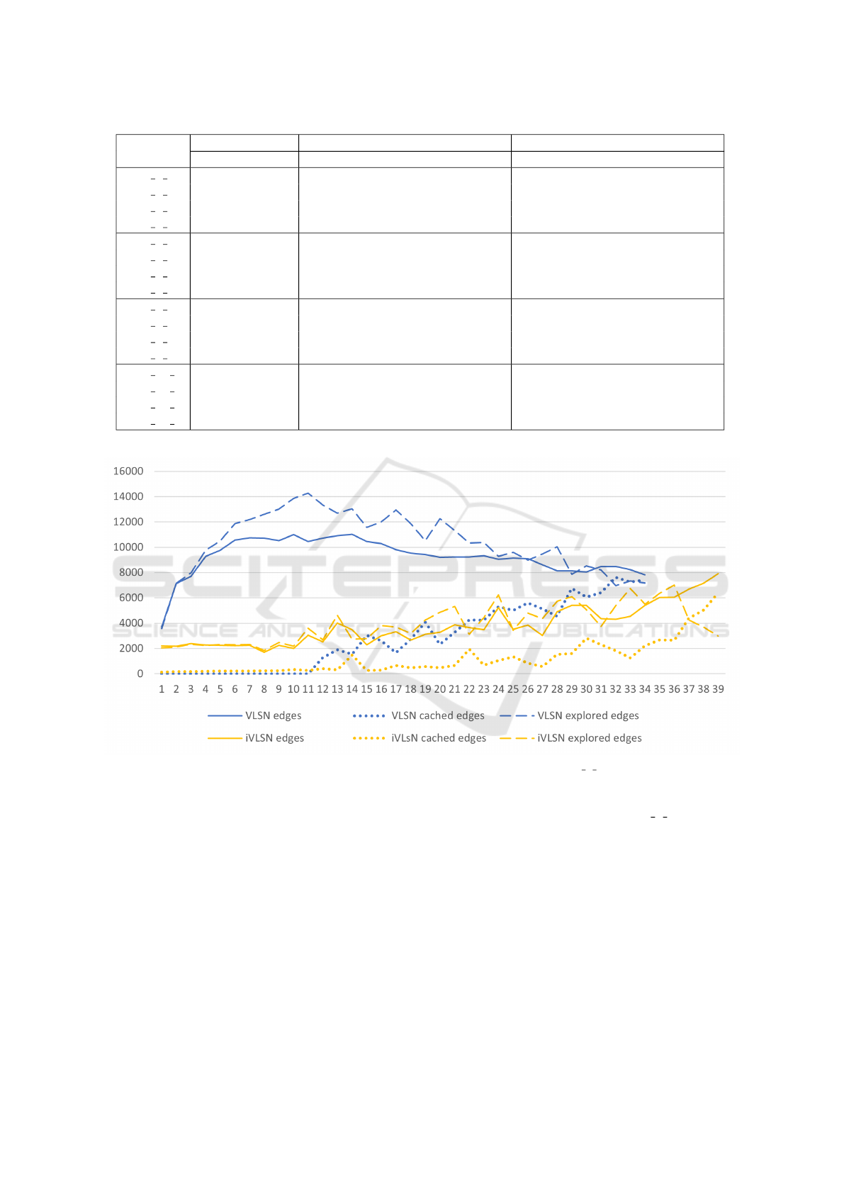
We compare the inner behaviour of VLSN and

iVLSN on a single run of the algorithms on the

LC1 2 4 problem instance in Figure 6. At each itera-

tion of the algorithm, it reports for both algorithms (1)

the number of edges in the VLSN graph and (2) num-

ber of such edges that were fetched from the cache

and (3) the number of edges that were explored. In

this problem instance, VLSN and iVLSN took nearly

the same number of iterations: 34 and 39, respec-

tively.

At any time, iVLSN explores fewer edges than

VLSN. In total, iVLSN explores 43% of the edges

explored by VLSN. The total run time of iVLSN is

53% of the time taken by VLSN. The gain in time is

not as high as the gain in number of edges because

the iVLSN executes the cycle detection algorithm per

iteration and performs a few more iterations in this

case.

After a start-up phase, where the VLSN injects

many pick-up-delivery pairs into the route, the total

number of edges explored by the VLSN decreases

throughout the search because the cache is more and

more effective. The iVLSN has the opposite be-

haviour; it explores more and more edges throughout

ICORES 2021 - 10th International Conference on Operations Research and Enterprise Systems

278

instance best known VLSN iVLSN

v obj best v obj of best v best obj best v obj of best v best obj

LC1 2 1 20 2704.57 21 2849,32 2704,68 22 2895,67 2704,68

LC1 2 2 19 2764.56 24 3362,84 2892,52 20 2817,33 2817,33

LC1 2 3 17 3127.78 21 3201,37 2772,29 19 2921,03 2772,29

LC1 2 4 17 2693.41 20 2899,35 2718,60 19 2716,54 2715,60

LC1 4 1 40 7152.06 44 7733,35 7285,22 42 7426,48 7152,27

LC1 4 2 38 8007.79 41 7369,02 7365,83 45 8184,20 7176,45

LC1 4 3 32 8678.23 42 8060,48 7550,04 39 7493,85 7436,44

LC1 4 4 30 6451.68 39 7493,27 7263,72 36 7191,33 7121,61

LC1 8 1 80 25184.38 86 27189,09 25874,91 82 25687,15 25184,82

LC1 8 2 76 30603.57 83 26203,90 26095,75 80 25589,06 25589,06

LC1 8 3 63 26430.39 80 27456,01 26812,03 77 26697,61 25769,06

LC1 8 4 59 22686.08 72 25297,93 24935,62 68 24367,39 24283,83

LC1 10 1 100 42488.66 103 43639,52 42489,22 103 43913,51 42489,22

LC1 10 2 94 44548.51 103 46200,78 44422,54 101 44247,74 43018,71

LC1 10 3 79 44692.86 97 44466,82 43880,41 96 44364,91 43483,82

LC1 10 4 73 37515.04 93 43615,39 41989,41 86 41082,67 40494,08

Figure 5: Comparing VLSN and iVLSN against the best known solutions.

Figure 6: Comparing internal metrics of VLSN and iVLSN on LC1 2 4.

the search, because cycles become harder to ﬁnd.

The iVLSN algorithm generates a VLSN graph

with fewer edges than the graph generated by the

VLSN algorithm, except for the very last value of

each algorithm, where these two numbers are equals

because the iVLSN must build the full graph to check

that no cycle exist in it.

Finally, more edges are fetched from the cache by

VLSN than iVLSN, simply because iVLSN just does

not populate the graph as much as VLSN, hence less

edges can be stored in the cache.

More benchmarks must be performed to compare

the iVLSN algorithm against the best results reported

in (Li and Lim, 2001). So far, we hope that iVLSN

can constitute a decent time/quality trade-off for small

problem instances such as the LC1 2 X instances,

considering that the best solutions for these instances

are generally generated with a run time of 15 minutes

(Curtois et al., 2018).

6 CONCLUSION

This paper presented a VLSN approach to the

PDPTW problem. The approach could be applied

easily using a generic VLSN algorithm, instantiated

with PDP-speciﬁc neighbourhoods. The latter are

built as cross-products of standard routing neighbour-

A Very Large Scale Neighborhood Approach to Pickup and Delivery Problems with Time Windows

279

hoods.

A generic approach is proposed to speed up the

VLSN algorithm, based on incremental computa-

tion. It proceeds through a gradual enrichment of

the VLSN graph instead of a full construction of the

graph prior to cycle search. This provides a no-

table speed improvement on the PDPTW as illustrated

through the benchmarks. A marginal quality improve-

ment was also observed.

VLSN algorithms experience local minima, like

any local search methods. On the considered bench-

mark instances, it could not reproduce the best known

result for the standard PDPTW benchmarks (Lim,

2008). Yet for the small problem instance, it was

not too far off the best known value, with a relatively

small response time. More benchmarks must be per-

formed to compare the VLSN approach against the

best results reported in (Lim, 2008). So far, we hope

that VLSN can constitute a decent time/quality trade-

off at least for small problem instances.

To further improve the quality of the solutions,

VLSN requires additional meta-heuristics. They can

either be added around it, such as restarts, or added

within it, for instance by accepting composite moves

based on a simulated annealing acceptance criterion

(Mouthuy et al., 2011).

To further speed up VLSN, several approaches

might be considered, including:

• parallelizing the construction of the VLSN to ex-

ploit multiple hardware cores; the construction it-

self is easy to parallelize because each edge of

the VLSN graph is evaluated independently to

the others and requires some neighborhood explo-

ration with a minimal amount of work, so this may

compensate the overhead of parallelization.

• making the cycle detection algorithm incremental,

so that it would only search for cycles involving

at least one edge that was added since its previous

execution.

• ﬁne tune the number of edges that are explored

between each run of the cycle detection algorithm.

there is trade off to set as too many edges and lots

of them are not useful, too few, and fewer cycles

will be detected with an increased time overhead

caused by the cycle detection algorithm.

ACKNOWLEDGEMENTS

This research was supported by the SAMOBIGrow

CWALITY research project from the Walloon Region

of Belgium (nr. 1910032).

REFERENCES

Curtois, T., Landa-Silva, D., Qu, Y., and Laesanklang, W.

(2018). Large neighbourhood search with adaptive

guided ejection search for the pickup and delivery

problem with time windows. EURO Journal on Trans-

portation and Logistics, 7(2):151–192.

De Landtsheer, R., Guyot, Y., Ospina, G., and Ponsard,

C. (2016). Recent developments of metaheuristics,

chapter Combining Neighborhoods into Local Search

Strategies. Springer.

Dumas, Y., Desrosiers, J., and Soumis, F. (1991). The

pickup and delivery problem with time windows. Eu-

ropean Journal of Operational Research, 54(1):7 – 22.

Germeau, F., Guyot, Y., Ospina, G., Landtsheer, R. D., and

Ponsard, C. (2018). Easily building complex neigh-

bourhoods with the cross-product combinator. In Pro-

ceedings of ORBEL’32.

Glover, F. and Kochenberger, G. (2003). Handbook of

Metaheuristics. International Series in Operations Re-

search & Management Science. Springer US.

Li, H. and Lim, A. (2001). A metaheuristic for the pickup

and delivery problem with time windows. In Proceed-

ings 13th IEEE International Conference on Tools

with Artiﬁcial Intelligence. ICTAI 2001, pages 160–

167.

Lim, L. . (2008). Li & lim pdptw benchmark.

https://www.sintef.no/projectweb/top/pdptw/.

Mladenovic, N., Urosevic, D., Hanaﬁ, S., and Ilic, A.

(2012). A general variable neighborhood search

for the one-commodity pickup-and-delivery travelling

salesman problem. Eur. J. Oper. Res., 220(1):270–

285.

Mouthuy, S., Hentenryck, P. V., and Deville, Y.

(2011). Constraint-based very large-scale neighbor-

hood search. Constraints, 17:87–122.

Orlin, J. B., Ahuja, R. K., and Magnanti, T. L. (1993).

Network ﬂows: Theory, algorithms, and applications.

Prentice Hall.

OscaR Team (2012). OscaR: Operational research in

Scala. Available under the LGPL licence from

https://bitbucket.org/oscarlib/oscar.

Pesch, E. and Glover, F. (1997). Tsp ejection chains. Dis-

crete Applied Mathematics, 76(1):165 – 181. Second

International Colloquium on Graphs and Optimiza-

tion.

Scala (2020). The Scala programming language.

http://www.scala-lang.org.

ICORES 2021 - 10th International Conference on Operations Research and Enterprise Systems

280