As Plain as the Nose on Your Face?

Peter A. C. Varley

, Stefania Cristina

, Alexandra Bonnici

and Kenneth P. Camilleri

Department of Systems and Control Engineering, University of Malta, Msida MSD 2080, Malta

Keywords:

Gaze Tracking, Head Pose, Noses, Haar Cascades.

Abstract:

We present an investigation into locating nose tips in 2D images of human faces. Our objective is conference-

room gaze-tracking, in which a presenter can control a presentation or demonstration by gaze from a distance

in the range 2m to 10m. In a ﬁrst step towards this, we here consider faces in the range 150cm to 300cm. Head

pose is the major contributing component of gaze direction, and nose tip position within the image of the face

is a strong clue to head pose. To facilitate detection of nose tips, we have implemented a combination of two

Haar cascades (one for frontal noses and one for proﬁle noses) with a lower failure rate than existing cascades,

and we have examined a number of ”hand-crafted ferns” for their potential to locate the nose tip within the

nose-like regions returned by our Haar cascades

1 INTRODUCTION

Our objective is conference-room gaze-tracking, in

which a presenter can control a presentation or

demonstration by gaze from a distance in the range

2m to 10m.

Current gaze-tracking systems typically track the

gaze of a computer user, usually seated about 70cm

from the camera. Some interactive displays such as

(Zhang, 2016) assume that the user is 130cm from

the camera. In a ﬁrst step towards extending this, we

consider faces in the range 150cm to 300cm. Many

images from the Labelled Faces in the Wild dataset

(Huang et al., 2007), such as those in Figure 1, are

typical of faces in this range.

There are two components which combine to give

a gaze estimate: head pose, and eyeball rotation. In

this short paper, we deal only with head pose. The

geometry of combining head pose and eyeball rota-

tion to obtain a full gaze vector is well-known - see

(for example) (Ishikawa et al., 2004). Readers in-

terested in eyeball rotation and in gaze-tracking in

general may wish to consult (Cristina and Camilleri,

2018), and those interested in a comparison of differ-

ent face-ﬁnding methods may wish to consult (Rah-

mad et al., 2020).

Of the two, head pose is the major contributor, as

https://orcid.org/0000-0003-4181-9234

https://orcid.org/0000-0003-4617-7998

https://orcid.org/0000-0002-6580-3424

https://orcid.org/0000-0003-0436-6408

the head has a wider range of movement than the eye-

ball, and it is also easier to detect as the head is larger

and more visible. We may also wish to allow for a

failsafe mode in which we use head pose alone when

pupil gaze direction is unavailable - users may even

prefer this, as they can control the screen with head

pose while making eye contact with their audience.

Head pose can be estimated by locating and com-

bining facial features in an image, but which features

should be chosen? Some facial features are not even

visible in images from 10m away (irises are a few

pixels across at most, and pupils could disappear en-

tirely). And people talk in conference rooms, so mu-

table features such as the mouth are also unreliable.

The nose is part of the rigid structure of the head

- it is possible to gesture with the nose, but people do

not typically do so when giving presentations - and it

is proverbially the most visible feature of the face. In

this paper, we only consider methods which use the

nose (possibly in combination with other features) to

determine head pose.

Weidenbacher (Weidenbacher et al., 2006) uses

ten feature points to determine head pose: three from

each eye, the two nostrils, and the corners of the

mouth.

Fasthpe (Sapienza and Camilleri, 2014) uses the

nose tip and a triangle formed by eyes and mouth to

predict head pose. The principal advantage of this

over previous methods is that the nose tip is the fea-

ture furthest from the plane of the eyes and mouth,

so it is more informative about 3D than anything else.

Varley, P., Cristina, S., Bonnici, A. and Camilleri, K.

As Plain as the Nose on Your Face?.

DOI: 10.5220/0010315404710479

In Proceedings of the 16th International Joint Conference on Computer Vision, Imaging and Computer Graphics Theory and Applications (VISIGRAPP 2021) - Volume 4: VISAPP, pages

471-479

ISBN: 978-989-758-488-6

471

(a) (b) (c)

Figure 1: From LFW (a) Frontal Nose, (b) Proﬁle Nose, (c) Ambiguous Nose.

A further advantage is that there is only one calibra-

tion parameter needed, distance of nose tip from eye-

mouth plane, and it has an obvious geometric mean-

ing and is easily and unobtrusively determined for a

new user. On the other hand, although ﬁtting a tetra-

hedron to four points is straightforward, it is not ro-

bust to bad points.

Our planned system will make use of both eye

gaze direction and head pose, and we follow Fasthpe

in using the nose tip to determine head pose. For this,

we need an accurate position of the nose tip in the

image. This paper considers various methods of de-

termining the nose tip position, makes recommenda-

tions, and presents preliminary results.

This paper does not discuss how to convert nose

tip position to a gaze prediction. This is something we

shall test in due course. Options range from simply

projecting a vector from a reference point to the nose

tip, as in Figure 2, to compiling a feature vector (a list

of facial landmarks and their locations) and using this

as an auxiliary input to a neural network, as in (Lu and

Chen, 2016) and (Zhang, 2016), or even to creating a

full 2.5D head model (Caunce et al., 2009).

Ergonomically, any strictly monotonic function

which converts a nose tip position to a gaze predic-

tion is potentially satisfactory, and indeed it is pos-

sible that users may prefer to make exaggerated ges-

tures rather than geometrically-accurate gestures.

On a practical note: we prefer methods which can

be retrained quickly on a portable computer. Should

it happen that a demonstration fails in the morning

(which is always possible with a prototype), we would

wish to gather training data from our potential cus-

tomers during the coffee break, add this to our training

dataset, retrain the system over the lunch break, and

demonstrate a working system in the afternoon, all

without having to return to the laboratory to use com-

puters with more parallel processing capability but no

mobility.

We also prefer methods which are easily repli-

cated: other researchers should be able to reproduce

(or even improve on!) our results.

Section 2 describes the characteristics of noses in

images of human faces. Section 3 lists and discusses

previous work. Section 4 describes our own investi-

gations to date and presents preliminary results. Sec-

tion 5 presents our conclusions and plans for further

development of our ideas.

1.1 Terminology

By convention, left and right are from the user’s point

of view, so the left eye and left nostril are those on the

right of the image.

2 NOSES IN IMAGES

The three images in Figure 1 are taken from the LFW

Dataset (Huang et al., 2007). This is a reasonable

source of training data: images are 250x250, the face

of the subject is usually central, and the size of the

face is usually between 60x60 and 130x130 pixels,

with the median being 110x110. Such images would

be typical of a webcam image of a subject at a dis-

tance of between 1.5m and 3m.

We maintain two datasets. Our reference dataset.

used for testing, comprises 3007 sample images (1474

female, 1533 male) selected from the LFW dataset

such that each image portrays a different person;

some images contain additional faces in the back-

ground, and where these are detected too, they are

included in our test results. Our primary dataset is a

subset of 100 images (51 female, 49 male) taken from

the reference dataset and used during development -

the three images in Figure 1 are among those included

in our primary dataset. A total of 502 images, includ-

ing all of those in the primary dataset, have been fully

labelled by eye. Both primary and reference datasets

include wide varieties of lighting intensities and di-

rections.

VISAPP 2021 - 16th International Conference on Computer Vision Theory and Applications

472

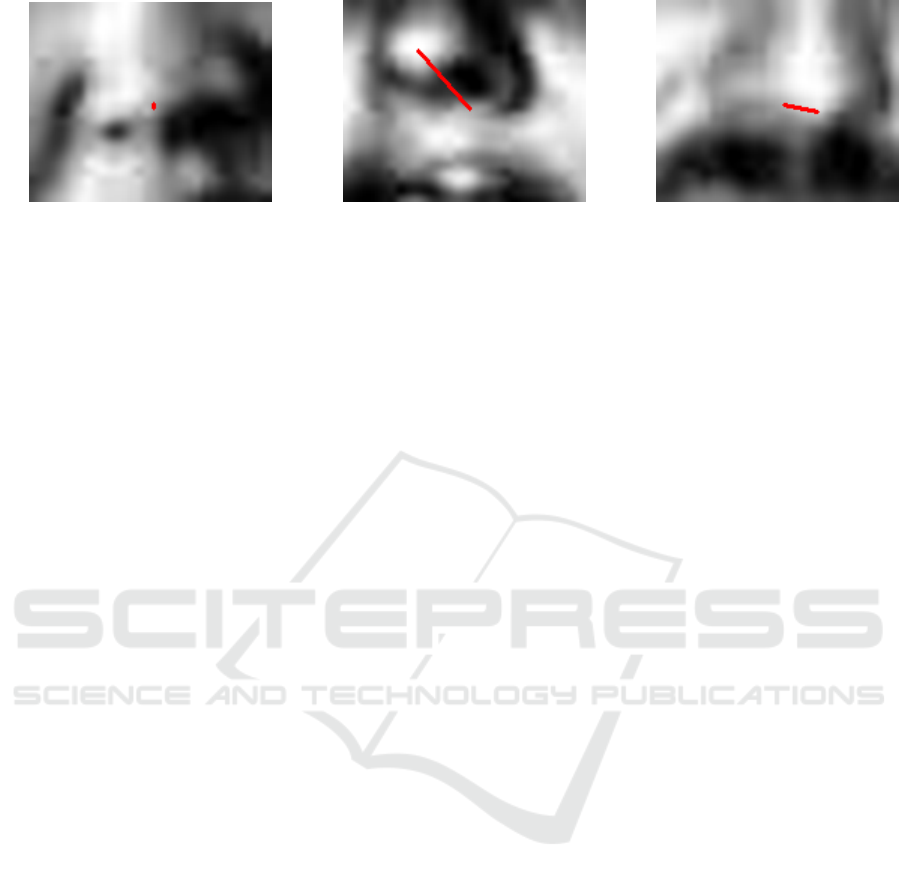
(a) (b) (c)

Figure 2: Nose Regions produced by MCS Nose Cascade from images in Figure 1.

It can be seen that in all three the nose gives a

good estimation of the head pose, and the head pose

gives a good estimation of the gaze. Even in more

complex cases where the eye direction and the head

pose are not in agreement, the head pose is still the

major component of the gaze direction, and we can

still obtain a good estimate of it from the nose.

Unlike eyeballs, which are always roughly spher-

ical so present the same appearance from any view-

point, noses are a peculiar and distinctive shape -

frontal noses (e.g. Figure 1a) and proﬁle noses (e.g.

Figure 1b) can look very different in 2D images. And

what are we to make of Figure 1c, which is mid-way

between frontal and proﬁle? Perhaps we can turn this

difﬁculty into an advantage - an accurate assessment

of where the nose is pointing will give us a very good

estimate of head pose.

3 METHODS

There are several established methods for detect-

ing features in images. Use of Haar Cascades is

widespread, not least because of their inclusion in

OpenCV (OpenCV, 2015). In recent years, Ferns

(Cao et al., 2012) have become popular.

3.1 Haar Cascades

Haar Cascades were introduced by (Viola and Jones,

2004), who described their innovation as “reminis-

cent of Haar basis functions”, with additions and im-

provements by (Lienhart and Maydt, 2002), who cre-

ated one of the most successful cascade classiﬁers, the

“alt2” face detector.

The simplest form of Cascade Classiﬁer is a lin-

ear sequence of Stage Classiﬁers (Viola and Jones,

2004). The number of Stage Classiﬁers is speciﬁed by

the user, and is typically around 20 (OpenCV, 2015),

(Castrill

on et al., 2007).

Each Stage Classiﬁer is a Haar Feature, a function

which compares the sums of pixel intensities in adja-

cent rectangles. There are ﬁve basic Haar Features

(Viola and Jones, 2004): four of these use 2 rectan-

gles; the ﬁfth uses 4. Tilted features at 45

◦

(Lien-

hart and Maydt, 2002) and symmetrical features can

be added if needed. To speed up this process, (Vi-

ola and Jones, 2004) introduced “intensity images”,

two-dimensional arrays in which each element con-

tains the sum of the intensities of pixels above and to

the left of that point in the original image; thus, calcu-

lating (T L +BR)−(T R +BL) from the four points at

the corners of a rectangle in the intensity image gives

the sum of all pixels in the the same rectangle in the

original image. Haar Features are weighted accord-

ing to their success at accepting positive samples and

rejecting negative samples.

Stages after the ﬁrst use Adaptive Boosting (Vi-

ola and Jones, 2004), in which successful Haar Fea-

ture/sample results in earlier stages are given a re-

duced weight when creating later stages, as their

job has already been done. Haar Cascades have

been used successfully to detect faces in images

(OpenCV, 2015) and to detect eyes and mouths in

faces (OpenCV, 2015), (Castrill

on et al., 2007).

One would think that, as noses are a peculiar and

distinctive shape, it should be easy to train Haar cas-

cades to ﬁnd them, as that is the sort of thing which

Haar cascades are good at. It is not so easy in practice.

For example, Castrill

on’s ”MCS” Haar nose cascade

(Castrill

on et al., 2007) is not reliable, possibly be-

cause of the decision to use 18x15 pixel samples - we

believe that this is too small. Its unequivocal success

rate is below 50% for the reference dataset described

above, as even when it ﬁnds exactly one “nose”, it

might be an eye, a forehead or a cheek rather than a

nose.

By adding common-sense pruning rules (the nose

is the one below the eyes and above the mouth) it is

possible to improve the success rate.

Table 1 shows the number of regions found by

the MCS nose cascade both without and with prun-

ing rules. It should be remembered that the num-

ber of nose-like regions found is an upper bound on

the number of successes, and the true number of suc-

cesses is lower, as we shall see in Section 4.

As Plain as the Nose on Your Face?

473

Table 1: Results (MCS cascade).

Regions MCS MCS & pruning

0 545 545

1 2361 2720

2 343 15

3 29 -

4 2 -

When successful, the MCS nose cascade typically

returns a rectangle which is 30% of the width and 25%

of the height of the face. The mid-point is typically

60% down from the top of the face. Resolving any

remaining ambiguity by choosing the one nearest this

ideal position is usually correct.

The images in Figure 2 were the nose regions re-

turned by applying the MCS nose cascade to Figure 1

(blurred to remove speckling). As the red lines super-

imposed on these images show, for frontal noses, the

nose tip is close to the centre of the nose region, but

for proﬁle noses, it is not; this is typical. Statistically,

the rule that the nose tip can be found at the centre

of the nose region is reasonably reliable, but the cases

where it fails are those where it is needed most.

In assessing the reliability of nose tip predictions,

we compare the prediction with our known nose la-

bellings. Errors of ±1 pixel in any direction are to

be expected and count as success. Errors of up to ±4

pixels are regarded as “near misses” - the method has

found the correct area but has not located it accurately.

Errors greater than ±4 pixels suggest that the method

has not found the correct area and are regarded as fail-

ure. Of our labelled images, the centres of the nose-

like regions found by the MCS nose cascade, pruned

as described earlier, are: 146 (29%) successful, 277

(55%) near misses, and 79 (16%) failures.

If Haar cascades are to be used for ﬁnding nose

tips, it seems necessary to treat frontal and proﬁle

noses separately, but this is not always straightfor-

ward. Sometimes, the distinction between frontal and

proﬁle noses is clear. Figure 1a is clearly frontal. Fig-

ure 1b is clearly proﬁle. But what of Figure 1c? We

classify this as a proﬁle nose, as part of the nose fea-

ture is self-occluded, but in terms of its general ap-

pearance, it looks more like a frontal nose.

3.2 Random Ferns

A Fern (Ozuysal et al., 2010) is a hint as to the likely

location of a feature. Individual ferns need not be re-

liable - as long as there are many of them and they

are mutually independent, the consensus is reliable

(Cao et al., 2012). Cao recommends Ferns chosen

at random, with the area from which they are chosen

shrinking gradually as the estimate of the position of

the feature improves.

The conceptual similarities between Haar Fea-

tures and Ferns are clear: both are weighted sums

of pixel intensity difference operations (2 or 3 such

operations for Haar Features, a conﬁgurable number,

optimally 5, for Ferns).

The main differences between Haar Features and

Ferns are:

• Haar Features are intended for use in sequences,

to take advantage of adaptive boosting; Ferns

are intended for use concurrently, using a voting

method to choose between their various predic-

tions

• Haar Features are created and analysed systemati-

cally; Ferns are drawn from an initial pool chosen

randomly. (As a consequence, creation of Fern is

much faster.)

• The chosen pixels in Ferns can be anywhere; the

chosen pixel sums in Haar Features are always

those of adjacent rectangles. (As a consequence,

Ferns are more ﬂexible.)

• The chosen pixels in Ferns can even be in other re-

gions of the image; the chosen rectangles in Haar

Features are always within the feature patch.

• Ferns are chosen according to their performance

in positive samples; Haar Features are chosen ac-

cording to their performance in both positive and

negative samples.

We argue that, while both methods have advan-

tages and disadvantages, it is clear which is which. If

speed is crucial, the exhaustive analysis of Haar Fea-

tures is a disadvantage, but the use of adaptive boost-

ing is an advantage. The ﬂexibility of Ferns is a clear

advantage over the inﬂexibility of Haar Features, but

Cao’s choice of including pixels from other regions of

the image in Ferns makes them vulnerable to changes

of lighting conditions, so is a disadvantage. And the

use of negative as well as positive samples when eval-

uating Haar Features is clearly beneﬁcial.

Thus, while Haar Features have their deﬁciencies,

abandoning them entirely in favour of Cao’s approach

is not the way to go.

We might also add a theoretical objection to Cao’s

idea. It is true that, as the initial pool of Ferns was cre-

ated randomly, they are mutually independent. But

the selection process is not random, it is based on

image data, and this introduces mutual dependence

within the ﬁnal pool of selected Ferns, and we can-

not guarantee that a consensus of mutually dependent

recommendations is better than any individual recom-

mendation. We shall return to this idea in the next

section.

VISAPP 2021 - 16th International Conference on Computer Vision Theory and Applications

474

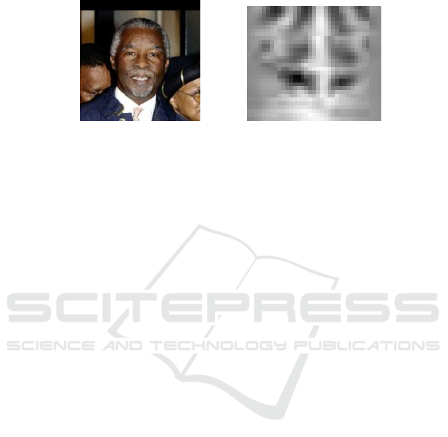
(a) (b)

Figure 3: A Symmetrical Nose (a) Original Image, (b) Self-Symmetry Output.

3.3 Hand-crafted Ferns

“Hand-crafted” ferns are the product of intelligent

observation rather than random selection (and (Cao

et al., 2012) deprecates their use for this reason). To

some extent, they can be considered to be related tech-

niques in the same general category as Haar Cascades

and Random Ferns, inheriting the best aspects of both:

as self-contained units, they can be used in sequence

or in parallel; their creation and analysis can be as sys-

tematic as their designer chooses; and while rectangu-

lar groups of pixels are faster to process than random

pixels, the rectangles need not be adjacent.

In this section, we discuss some ideas. Implemen-

tation recommendations and numerical results are to

be found in Section 4.

One idea which could ﬁnd the nose tip is simply

to pick the brightest part of the nose region, on the

reasoning that as the nose sticks out furthest from the

face plane, it is most likely to catch the light, as can

be seen in Figures 2b and 2c.

Working on the same lines, the brightness gradient

down from the tip of the nose should be steepest, as

the base of the nose is occluded and dark. This is still

vulnerable to teeth and cheeks, and if the nose region

is too large, it can even detect the white of the eye.

A related idea is to locate nostrils at the darkest

two patches of the region and work from there. Pre-

liminary results suggest that this is very sensitive to

lighting conditions. One of the nostrils is usually the

darkest patch in the region. For frontal noses, the

second-darkest area could be anywhere - there is no

consistency. For proﬁle noses, the second-darkest re-

gion is so often the shadow of the wing of the darker

side of the nose (as can be seen in Figure 2b) that this

could be used as a reliable clue to the nose structure.

A combination of the previous two ideas, in which

we compare the brightness of a single region with the

darkness of two regions diagonally below it, has been

found to be more successful than either.

For completeness, we also analysed a number of

other options, the most successful of which was the

inverse idea, comparing the brightness of a single

region with the darkness of two regions diagonally

above it. This too has merits - the depressions diago-

nally above the nose tip fail to catch the light.

The above ideas are clearly not mutually indepen-

dent, as they all start by assuming a bright area (abso-

lute or relative) around the nose tip. Ideally, we would

wish to combine one or more of these with unrelated

methods.

One independent idea would be to ﬁnd the x-

coordinate of the nose tip by ﬁnding a vertical plane

of mirror symmetry through the nose region. Where

the subject of the image has a particularly symmetri-

cal nose (such as Figure 3a), self-symmetry of pixel

intensities gives useful results (a clear, almost-vertical

line can be seen in Figure 3b). However, this idea is

particularly sensitive to lighting conditions and can-

not be recommended.

We have also experimented with using self-

symmetry of intensity gradients rather than self-

symmetry of intensities. This was unsuccessful and

has nothing to recommend it.

3.4 Other Methods

Artiﬁcial intelligence methods such as Convolutional

Neural Networks could be used very effectively, as

taking account of subtle cues elsewhere in an image

is what they are good at, but using a CNN just to ﬁnd a

nose tip seems like overkill - ﬁnding the nose tip will

be just one small component (albeit the most difﬁcult

to implement) of a much larger system.

Furthermore, the advantages of CNNs do not com-

pensate for the practical disadvantage mentioned in

Section 1. Retraining CNNs is slow and resource-

intensive, often requires multiple-processor hardware,

and can take hours or even days. For our purposes, a

system which takes 30 minutes to retrain on a lap-

top computer and works adequately thereafter is bet-

ter than a system which may work somewhat better

As Plain as the Nose on Your Face?

475

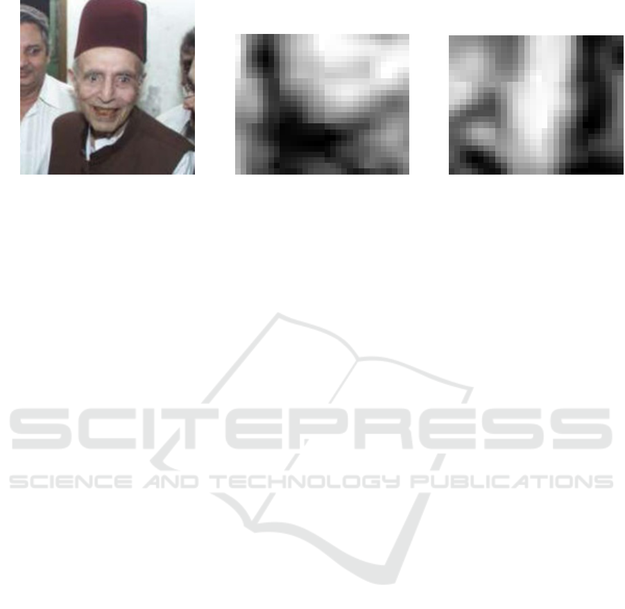
(a) (b) (c)

Figure 4: Problematic Face (a) Original Image, (b) Not a Nose (MCS), (c) Frontal Nose.

but could require 30 hours, or specialist hardware, or

both.

4 INVESTIGATION

We have trained our own nose cascades using images

taken from the LFW dataset and labelled by eye. We

trained two cascades using positive samples with the

nose tip at the centre, one for frontal noses and one

for proﬁle noses (using symmetrical cascades so as

to allow for both left-facing and right-facing proﬁle

noses).

The frontal face cascade is sized at 25x17 pixels

(see Section 4.1). It was created using 276 positive

and 648 negative samples. It has 16 stages. It took 37

minutes to create on a home laptop. The proﬁle face

cascade is sized at 35x19 pixels - it is larger as it may

have to contain the whole nose in little more than half

of its region. It was created using 155 positive and

533 negative samples. It has 18 stages. It took 78

minutes to create on a home laptop.

When creating cascades, we used the entire pri-

mary dataset, plus additional images from the refer-

ence dataset as required to improve cascade perfor-

mance. As labelling was by eye, nose tip position is

often subjective and errors of ±1 pixel are to be ex-

pected.

Builds are tested initially using the primary

dataset, and successful builds are then tested more

thoroughly using the reference dataset.

In addition, we have a “rogue’s gallery” of 10

faces (4 female, 6 male, including Figures 4a and 5a)

which were particularly troublesome during develop-

ment and which received special attention. These do

not overlap with the primary dataset.

Numerical results for these cascades are to be

found in Section 4.2. It is clear that, when both frontal

and proﬁle cascades ﬁnd the same region, we need a

better way of combining the two predictions, as either

cascade alone is better at locating the nose tip than is

combining the two.

While we were developing our cascades, it was

the face shown in Figure 4a which gave the most false

positives, both before and after pruning. MCS (Cas-

trill

on et al., 2007) ﬁnds just a single “nose” region

for this face, the one shown in Figure 4b - unfortu-

nately, however nose-like it may appear, this is his

right cheek. The real nose, shown in Figure 4c, is one

of several nose-like regions found by our cascades.

The face shown in Figure 5a is the one which

currently gives the most false positives after pruning.

MCS (Castrill

on et al., 2007) ﬁnds two “nose” regions

for this face, but the false one is pruned out, leav-

ing the region shown in Figure 5b. Our cascades ﬁnd

more possibilities, including not only the one in Fig-

ure 5b but two in which one nostril and one fold of

the cheek are interpreted as two nostrils, as shown in

Figure 5c.

Even knowing that the nose is on the right-hand

side of Figure 5c, it is hard not to interpret the feature

on the left-hand side of the image as a second nose.

Pruning cheeks is not straightforward. Most of

them lie within a bounding box formed from the out-

side edges of the eye regions and the edges of the

mouth region, and many of them even lie within a

bounding box formed from the centres of the eye re-

gions and the edges of the mouth region. Shrinking

the bounding box further could exclude many genuine

noses.

Since our cascade combination ﬁnds the correct

nose position (albeit alongside many false positives)

and MCS does not, the result for Figure 4 must be

counted as a modest success. But there is clearly

much more work still to be done before we have a

reliable nose-ﬁnder.

4.1 Cascade Region Size

In support of our belief that 18x15 pixels is too small,

we offer the following analysis for frontal noses.

We created three frontal nose cascades, using the

VISAPP 2021 - 16th International Conference on Computer Vision Theory and Applications

476

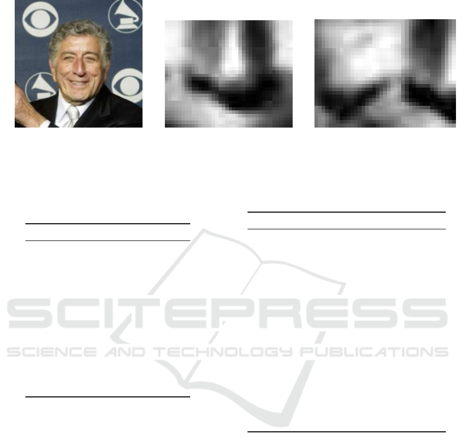
(a) (b) (c)

Figure 5: Problematic Face (a) Original Image, (b) Nose Region (MCS), (c) Two Noses?

same 276 positive and 648 negative samples. The cas-

cades were sized at 19x13, 25x17 and 31x21 pixels.

The numbers of nose-like regions found by each of

these cascades are shown in Table 2.

Table 2: Frontal Nose Cascades.

# Regions 19x13 25x19 31x21

0 1260 480 391

1 1275 985 452

2 562 879 569

3 157 551 568

4 22 241 468

5 4 106 359

6 - 29 211

7 - 9 138

8 - - 66

9 - - 30

10 - - 17

11 - - 9

12 - - 2

Clearly, using larger patch sizes reduces the num-

ber of failures but increases the number of false pos-

itives. Our feeling is that 25x17 is optimal, and we

hypothesise that this is because it is the typical size of

noses in the LFW dataset - smaller sample sizes lose

information, but larger sample sizes do not gain much

information.

The effects on system performance will have to

be tested during integration - perhaps, in our ﬁnal

system, we should have several cascades of differ-

ent sample sizes prepared in advance, and choose be-

tween them according to the size of the face.

4.2 Combined Cascade Performance

Table 3 shows the numbers of nose-like regions found

by (a) our proﬁle nose cascade alone, (b) the com-

bination of frontal and proﬁle nose cascades without

pruning, and (c) the combination with pruning. The

key result is that the number of images with 0 nose-

like regions is less than half of that using the MCS

cascade.

Table 3: Proﬁle and Combined Nose Cascades.

# Regions Proﬁle Combined + Pruning

0 414 263 263

1 765 215 632

2 841 419 1832

3 642 552 443

4 363 512 87

5 178 453 22

6 49 324 1

7 23 242 -

8 4 140 -

9 1 88 -

10 - 47 -

11 - 13 -

12 - 7 -

13 - 3 -

14 - 1 -

15 - 0 -

16 - 1 -

4.3 Hand-crafted Ferns

We analysed the performance of a number of

multiple-boxcar methods, all of which sum pixel in-

tensities in square patches, and compared their per-

formance with the simple ideas presented above. In

order to ensure that they are independent of light-

ing conditions, we limited our investigations to pixel-

intensity-difference operations (reducing dependence

on lighting intensity) between boxcars which are (a)

in horizontally-symmetrical patterns (reducing de-

pendence on lighting direction) and (b) in which the

brightest region spans the line of symmetry (regard-

less of lighting, the nose tip protrudes furthest from

the face plane and will catch the light best). We

present them in ascending order of complexity. Box-

As Plain as the Nose on Your Face?

477

car sizes are optimised for 250x250 images in which

the face is about 110x110 pixels, and should be varied

in proportion for larger or smaller faces. Results were

obtained using combined frontal and proﬁle nose cas-

cades, with pruning, and 502 labelled noses.

Fern C is the idea already presented: the nose tip

is at the centre of the region found by the Haar cas-

cades. Of our 502 labelled noses, 153 (29%) were

successful, 205 (39%) were near misses, and 144

(29%) were failures.

Fern B is a single boxcar: we ﬁnd the brightest 9x9

square in the nose region. The nose tip is 7 pixels be-

low the centre of the square. This Fern is based on the

assumption that the nose tip will catch the light as it

sticks out. Of our labelled noses, 67 (13%) were suc-

cessful, 189 (38%) were near misses, and 246 (49%)

were failures.

Fern D is a double-boxcar: we ﬁnd the pair of 7x7

squares M and N where M is immediately above N

which maximises (ΣM − ΣN). The nose tip is 2 pix-

els below the centre of M. This Fern is based on the

assumption that the bottom of the nose will usually

be dark as lighting is usually from above. Of our la-

belled noses, 98 (20%) were successful, 147 (29%)

were near-misses, and 257 (51%) were failures.

Fern V is a vertical triple-boxcar: we ﬁnd the trio

of 7x7 squares L, M and N where M is immediately

below L and immediately above N which maximises

(2ΣM − ΣL − ΣN). The nose tip is 3 pixels below

the centre of square M. The assumption behind this

Fern is that even if the nose tip is not bright in abso-

lute terms, it will nevertheless be brighter than its sur-

roundings. Of our labelled noses, 87 (17%) were suc-

cessful, 123 (25%) were near misses, and 292 (58%)

were failures.

Fern H is a horizontal triple-boxcar: we ﬁnd the

trio of 9x9 squares L, M and N where L and N

are immediately either side of M which maximises

(2ΣM − ΣL − ΣN). The nose tip is at the centre of

M. The assumption behind this Fern is that even if

the nose tip is not bright in absolute terms, it will be

bright relative to its surroundings. Of our labelled

noses, 57 (11%) were successful, 101 (20%) were

near-misses, and 344 (69%) were failures.

Fern T is a triangular triple-boxcar: we ﬁnd the

trio of 7x7 squares L, M and N where the centres of

L and N are 3 pixels below and 4 pixels either side of

the centre of M which maximises (2ΣM − ΣL − ΣN).

The nose tip is at the centre of square M. This method

is based on the assumption that nostrils are dark and

are to be found either side of, and slightly below, the

nose tip. Of our labelled noses, 185 (37%) were suc-

cessful, 169 (34%) were near-misses, and 148 (29%)

were failures. Fern T is by far the best of those based

around a central bright square.

Fern U is an inverted triangular triple-boxcar: we

ﬁnd the trio of 11x11 squares L, M and N where the

centres of L and N are 7 pixels above and 9 pix-

els either side of the centre of M which maximises

(2ΣM − ΣL − ΣN). The nose tip is 6 pixels below the

centre of square M. This fern is based on the assump-

tion that the depressions in the sides of the nose will

be darker than their surroundings as they do not catch

the light. Of our labelled noses, 61 (12%) were suc-

cessful, 183 (36%) were near-misses, and 258 (52%)

were failures.

Ferns are intended to be used together, and it is

their team performance which is most important.

We combined the predictions of the two most

successful ferns, C and T , using a weighted mean.

We might expect both advantages and disadvantages:

where one fern is right and the other is wrong, com-

bining the two will be detrimental, but it can also hap-

pen that the two predictions are near-misses in oppo-

site directions, and combining them results in an ac-

curate prediction. In practice, the results are no better

and no worse at accurate prediction than Fern T (al-

though the binary prediction is slightly better at con-

verting failures to near-misses): 185 (37%) are suc-

cessful, 173 (34%) are near-misses, and 144 (29%)

are failures.

What we want is a neutral arbiter to adjudicate

those cases where the predictions of Ferns C and T

are signiﬁcantly different. Unfortunately, this is what

we lack: all of our other Ferns are biased towards Fern

T, as they all assume a bright square around the nose

tip.

In terms of individual performance, the next-best

Ferns are D and V , but these both include dark pix-

els below the nose which are also included in Fern T.

They are not neutral arbiters. Thus the ternary combi-

nation we tested combined Fern C with Ferns T and

U; these two may share the same bright region, but

the dark regions do not overlap.

The three predictions were combined as follows:

(a) weight all predictions according to how reliable

the method is; (b) ﬁnd the weighted mean of all pre-

dictions; (c) reweight the predictions according to

how close they are to the mean; and (d) recalculate

the weighted mean using the recalculated weights.

The results showed a slight decrease in accurate

prediction, but an increase in near-misses: 180 (36%)

were successful, 183 (36%) were near-misses, and

137 (27%) were failures. This can be explained as

the third fern doing its job successfully when the two

leading ferns make widely-different predictions, but

contributing its own (worse) prediction when the two

leading ferns are already close.

VISAPP 2021 - 16th International Conference on Computer Vision Theory and Applications

478

For the time being, we recommend using either

Fern T alone (for speed), or combining this with Fern

C (for somewhat better ability to avoid failures). If

we are to make further progress, we need a new Fern

which is independent of both.

5 CONCLUSION

This remains work in progress: it raises more ques-

tions than it answers. Haar classiﬁers followed by

”hand-crafted ferns” can usually ﬁnd the nose tip, but

are there other, faster, more accurate or more reli-

able ways? Is the nose tip the best feature to detect,

or would other parts of the nose (bridge or nostrils)

be better? To what extent can the nose alone deter-

mine head pose? - occluded nostrils mean the user is

looking down, and prominent nostrils mean the user

is looking up, but can this variation be detected with

sufﬁcient accuracy to be useful?

To some extent, our boxcar method combines the

advantages of Haar Features and Random Ferns, but

as a ﬁrst attempt, it is unlikely to be optimal. A deeper

study would be welcome, but this would require a re-

turn to ﬁrst principles and is work for the future.

The results in Section 4 demonstrate that (a) our

combined cascade fails less often than MCS (Cas-

trill

on et al., 2007), and (b) it does not insist on a

wrong interpretation of problematic faces such as Fig-

ure 4a. This is progress. Nevertheless, there is clearly

much more work still to be done before we have a

reliable nose-ﬁnder.

The target for on-the-spot retraining has not been

met, particularly for proﬁle noses. While we are

waiting for faster portable computers to become

widespread, we may have to accept that on-the-spot

retraining is limited to frontal noses.

ACKNOWLEDGEMENTS

The authors wish to acknowledge the project: “Set-

ting up of transdisciplinary research and knowledge

exchange (TRAKE) complex at the University of

Malta (ERDF.01.124)”, which is co-ﬁnanced by the

European Union through the European Regional De-

velopment Fund 2014–2020.

REFERENCES

Cao, X., Wei, Y., Wen, F., and Sun, J. (2012). Face align-

ment by explicit shape regression. In CVPR, pages

2887–2894.

Castrill

on, M., D

eniz, O., Hern

andez, M., and Guerra, C.

(2007). Encara2: Real-time detection of multiple

faces at different resolutions in video streams. In Jour-

nal of Visual Communication and Image Representa-

tion Vol 18 No 2, pages 130–140.

Caunce, A., Cristinacce, D., Taylor, C., and Cootes, T. F.

(2009). Locating facial features and pose estimation

using a 3d shape model. In ISVC09.

Cristina, S. and Camilleri, K. P. (2018). Unobtrusive and

pervasive video-based eye-gaze tracking. In Image

and Vision Computing 74, pages 21–40.

Huang, G. B., Ramesh, M., Berg, T., and Learned-Miller,

E. (2007). Labeled faces in the wild: A database for

studying face recognition in unconstrained environ-

ments. Technical Report 07-49, University of Mas-

sachusetts, Amherst.

Ishikawa, T., Baker, S., Matthews, I., and Kanade, T.

(2004). Passive driver gaze tracking with active ap-

pearance models. In Proceedings of the 11th World

Congress on Intelligent Transportation Systems.

Lienhart, R. and Maydt, J. (2002). An extended set of haar-

like features for rapid object detection. In Proceed-

ings. 2002 International Conference on Image Pro-

cessing volume 1, pages I–900. IEEE.

Lu, F. and Chen, Y. (2016). Person-independent eye gaze

prediction from eye images using patch-based fea-

tures. In Neurocomputing (NC).

OpenCV (2015). Open Source Computer Vision Library.

Ozuysal, M., Calonder, M., Lepetit, V., and Fua, P. (2010).

Fast key-point recognition using random ferns. In

IEEE Transactions on Pattern Analysis and Machine

Intelligence,32(3), pages 448–461.

Rahmad, C., Andrie, R., Putra, D., Dharma, I., Darmono,

H., and Muhiqqin, I. (2020). Comparison of viola-

jones haar cascade classiﬁer and histogram of oriented

gradients (hog) for face detection. In IOP Confer-

ence Series: Materials Science and Engineering. 732.

012038.

Sapienza, M. and Camilleri, K. P. (2014). Fasthpe: A recipe

for quick head pose estimation. Technical Report TR-

SCE-2014-01, University of Malta.

Viola, P. and Jones, M. (2004). Robust real-time face de-

tection. In International Journal of Computer Vision,

57(2), pages 137–154.

Weidenbacher, U., Layher, G., Bayerl, P., and Neumann,

H. (2006). Detection of head pose and gaze direction

for human-computer interaction. In Perception and

Interactive Technologies. PIT.

Zhang, Y. (2016). Eye tracking and gaze interface design

for pervasive displays. PhD thesis, University of Lan-

caster.

As Plain as the Nose on Your Face?

479