Improved HTM Spatial Pooler with Homeostatic Plasticity Control

Damir Dobric

, Andreas Pech

, Bogdan Ghita

and Thomas Wennekers

University of Plymouth, Faculty of Sciences and Engineering, U.K.

Department of Computer Science and Engineering, Frankfurt University of Applied Sciences, Germany

Keywords: Hierarchical Temporal Memory, Corticallearning Algorithm, Spatial Pooler, Homeostatic Plasticity.

Abstract: Hierarchical Temporal Memory (HTM) - Spatial Pooler (SP) is a Learning Algorithm for learning of spatial

patterns inspired by the neo-cortex. It is designed to learn the pattern in a few iteration steps and to generate

the Sparse Distributed Representation (SDR) of the input. It encodes spatially similar inputs into the same or

similar SDRs memorized as a population of active neurons organized in groups called micro-columns.

Findings in this research show that produced SDRs can be forgotten during the training progress, which causes

the SP to learn the same pattern again and converts into the new SDR. This work shows that instable learning

behaviour of the SP is caused by the internal boosting algorithm inspired by the homeostatic plasticity

mechanism. Previous findings in neurosciences show that this mechanism is only active during the

development of new-born mammals and later deactivated or shifted from cortical layer L4, where the SP is

supposed to be active. The same mechanism was used in this work. The SP algorithm was extended with the

new homeostatic plasticity component that controls the boosting and deactivates it after entering the stable

state. Results show that learned SDRs remain stable during the lifetime of the Spatial Pooler.

1 INTRODUCTION

The Hierarchical Temporal Memory Cortical

Learning Algorithm (HTM CLA) is an algorithm

inspired by the biological functioning of the

neocortex, which combines spatial pattern

recognition and temporal sequence learning

(Hawkins, Subutai and Cui, 2017).

It organizes neurons in layers of column-like units

built from many neurons, such that the units are

connected into structures called areas. Areas,

columns and mini-columns are hierarchically

organized (Mountcastle, 1997) and can further be

connected in more complex networks, which

implement higher cognitive functions like invariant

representations, pattern- and sequence-recognition

etc. HTM CLA in general consists of two major

algorithms: Spatial Pooler and Temporal Memory.

The Spatial Pooler operates on mini-columns

connected to sensory inputs (Yuwei, Subutai and

Hawkins, 2017) . It is responsible to learn spatial

patterns by encoding the pattern into the sparse

distributed representation (SDR). The created SDR,

which represents the encoded spatial pattern is further

used as the input for the Temporal Memory (TM)

algorithm.

The TM is responsible for learning of sequences

from SDR. Experiments in this work show that the

current version of the Spatial Pooler is instable.

During the learning process, learned patterns will be

forgotten and learned again. Results show that the

Spatial Pooler oscillates between stable and unstable

stable. Moreover, experiments show the instability is

related to the single pattern and not to the set of

patterns.

For example, The Spatial Pooler can keep the

stable SDR1 for pattern p1 while SDR2 for pattern p2

becomes unstable and so on. Having stable Spatial

Pooler is essential for all applications that rely on

spatial pattern recognition. Because SDRs produced

by the Spatial Pooler are also used as an input for the

Temporal Memory algorithm, an unstable Spatial

Pooler will also cause the Temporal Memory

algorithm to forget learned sequences.

In this work, the instability of the SP was

investigated an extension (modification) of the

Spatial Pooler is proposed, which ensures the better

stability of the algorithm.

2 METHODS

To analyse the stability of the Spatial Pooler, an

instance of the SP with the set of common parameters

was created (see table 1).

Dobric, D., Pech, A., Ghita, B. and Wennekers, T.

Improved HTM Spatial Pooler with Homeostatic Plasticity Control.

DOI: 10.5220/0010314200980106

In Proceedings of the 10th International Conference on Pattern Recognition Applications and Methods (ICPRAM 2021), pages 98-106

ISBN: 978-989-758-486-2

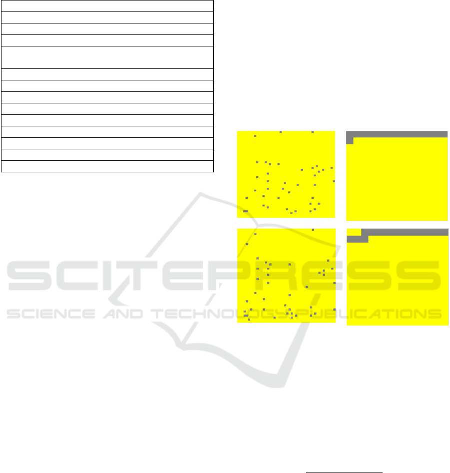
Table 1: Spatial Pooler parameters. Set of parameters

shown in the table are commonly used when working with

the Spatial Pooler.

Parameters Value

INPUT BITS 200

COLUMNS 2048

GLOBAL_INHIBITION true

NUM_ACTIVE_COLUMNS_PER_

INH_AREA

2% (40)

STIMULUS_THRESHOLD 0.5

SYN_PERM_INACTIVE_DEC 0.01

SYN_PERM_ACTIVE_INC 0.01

SYN_PERM_CONNECTED 0.1

MIN_PCT_OVERLAP_DUTY_CYCLES 0.001

MIN_PCT_ACTIVE_DUTY_CYCLES 0.001

POTENTIAL_RADIUS 1024

DUTY_CYCLE_PERIOD 100

MAX_BOOST 10

Most experiments were done with 2048 columns. In

this specific case, the scalar encoder was used to

encode input scalar values that are presented to the

Spatial Pooler during the learning process. As an

input, values between 0 and 100 were used. Before

presenting an input to the Spatial Pooler, every input

value was encoded with 200 bits, each value is

encoded with 15 non-zero bits. Figure 1 shows a few

examples of encoded scalar values.

For more detailed information about the meaning

of all parameters please see (Dobric, 2018).

The first row in Figure 1 represents the value ‘0’

and second-row the value ‘1’. The input value is on

right and the corresponding SDR is on left. Yellow

colour in the figure represents zero-bits and the grey

colour represents the non-zero bits. Grey dots on left

represent set of active columns after encoding of the

given input.

The Spatial Pooler algorithm implements a

boosting of columns inspired by homeostatic

plasticity mechanism (Turrigiano and Nelson, 2004),

(Davis and Graeme, 2006). This mechanism

influences excitation and inhibition balance of neural

cells and is likely important for maintaining the stable

cortical state. The functional stability of neural

circuits is achieved by homeostatic plasticity. It keeps

in balance the network excitation and inhibition and

coordinates changes in circuit connectivity (Tien and

Kerschensteiner, 2018).

Excitation mechanism in HTM is implemented

explicitly by algorithms Spatial Pooler and Temporal

Memory by setting cells inactive or predictive state.

Moreover, Spatial Pooler provides two inhibition

algorithms: Global Inhibition and Local Inhibition.

Inhibition algorithms control which cells around the

currently processing cell must be activated or

inhibited.

The boosting in the Spatial Pooler tracks the

column activity and makes sure that all columns are

uniformly used across all seen patterns. Because this

mechanism is continuously active, it can perform the

boosting of columns that already build learned SDRs.

Once that happens the Spatial Pooler will briefly

“forget” some learned patterns. If the forgotten

pattern is presented again to the SP, it will start

learning it again.

To analyse the learning behaviour of the Spatial

Pooler, a set of input patterns was presented to the SP

instance in many iteration steps.

Figure 1: Examples of two input values encoded by the

scalar encoder (right) and their corresponding Sparse

Distributed Representation (left) encoded by the Spatial

Pooler.

Every input pattern is encoded by Spatial Pooler into

SDR represented as a set of indices of active columns

𝐴



of the given pattern in the iteration k.

In every learning step of the same pattern, the

similarity between SDR in step k and the step k+1 is

calculated as shown in equation 1.

𝑠

𝐴



∩

𝐴



max |

𝐴



|, |

𝐴



|

(1)

The similarity 𝑠 is defined as a ratio between the

number of elements (cardinality) of the same active

columns in SDRs generated in steps k and k+1 and a

maximum number of active columns in two

comparing steps.

The Spatial Pooler is by definition stable if SDRs

of the same pattern does not change for the entire life

Improved HTM Spatial Pooler with Homeostatic Plasticity Control

cycle of the Spatial Pooler. In this case, the similarity

𝑠 between all SDRs of the same pattern is 100%.

Figure 2 shows the single input pattern presented

to SP in more than 25000 iterations.

Typically, Spatial Pooler learns patterns very fast.

It requires usually no more than two to three iterations

to learn the presented pattern. This behaviour is very

useful for real-life application because it does not

require a long training process.

Figure 2: Unstable Spatial Pooler. SP learns the pattern and

keeps the SDR unchanged for some iterations. When

boosting gets active SP forgets the SDR (similarity drops)

and starts learning again.

The y-axis shows the similarity s of SDRs in the

current iteration step and the previous step. The x-axis

shows the iteration step. The similarity of 100%

means the learned SDR does not change over time.

After an unspecified number of iterations, the SP

forgets the learned SDR and starts learning again.

Every time the SDR changes, it means the learned

SDR for that pattern is changed. Because the new

SDR for the pattern is created, the previously learned

one is forgotten. In that case, the similarity drops from

100% to zero or some other value. In contrast,

keeping the similarity on 100% means that learned

SDR for the same input is the same for the entire

iteration interval. If the similarity is less than 100%,

generated SDRs of the same input are different. This

indicates an unstable Spatial Pooler. As shown in

Figure 2 the learned state oscillates between stable

and unstable state during entire learning time, which

is not a useful behaviour for real-life applications.

This experiment clearly shows the instability of

the Spatial Pooler, but it does not show any details

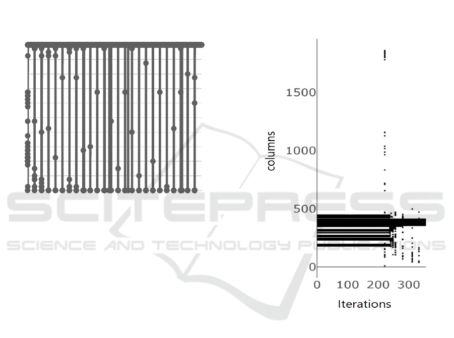
about the encoding of the SDR. Figure 3 shows the

same behaviour from a different point of view. It

shows how the SDR of the same pattern is encoded in

the first 300 iterations (cycles) on the example of a

single input value. The Spatial Pooler generates a

stable SDR right on the beginning of the learning

process and keeps it stable (unchanged) for approx.

200 iterations. After that SDR will change until the

Spatial Pooler enters the stable state again (not shown

in the figure) etc.

Figure 3: SDR shows active columns (SDR) of the learned

input in the first 300 iterations (cycles). The learned SDR is

unchanged (stable) in approx. first 200 iterations. After that,

it gets unstable.

In the next experiment, the boosting was disabled by

setting DUTY_CYCLE_PERIOD and

MAX_BOOST to zero value. These two values

disable boosting algorithm in the Spatial Pooler.

Results show that the SP with these parameters

produces stable SDRs as shown in Figure 4. The

figure shows an example of a stable encoding of the

single pattern with disable boosting algorithm. The

SP learns the pattern and encodes it to SDR in few

iterations (typically 2-3) and keeps it unchanged

(stable) during the entire life cycle of the SP instance.

By following this result, the stable SP can be

achieved by disabling of the boosting algorithm.

100

1667

3334

5001

6668

8335

10002

11669

13336

15003

16670

18337

20004

21671

23338

SDRsimilarityindependenceonthe

iterationstep

ICPRAM 2021 - 10th International Conference on Pattern Recognition Applications and Methods

100

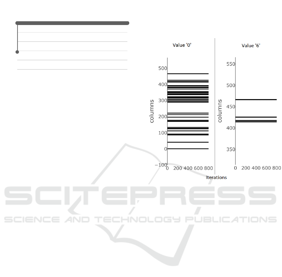
Figure 4: Spatial Pooler generates stable SDR after the

boosting is disabled.

Unfortunately, without the boosting mechanism, the

SP generates SDR-s with unpredictive number of

active mini-columns.

Figure 5 shows two input values ‘0’ and ‘6’. The

x-axis represents indexes of active mini-columns,

which participates in the encoding of the input value.

The y-axis represents the learning iteration. The SP is

stable if the SDR code does not change over time. As

already mentioned, disabling of boosting will cause

the SP to enter the stable state as shown in Figure 5.

The value ‘0’ is encoded with approx. 40 active

mini-columns and the value ‘6’ is encoded with 4

active mini-columns. This is a significant unwanted

difference. Experiments showed that some values can

even be encoded without any active mini-column if

boosting is disabled.

If the number of active mini-columns in an SDR

for different inputs is significantly different, the

further processing of memorized SDR-s will be

negatively influenced. Most operations in the

Hierarchical Temporal Memory rely on the

calculation of the overlap between neural cells,

synapses or mini-columns (Subutai, Hawkins, 2016).

In that case, SDR-s with the much higher number of

active columns will statistically produce higher

overlaps, which is not in balance with other SDR-s

with less active cells.

The parameter NUM_ACTIVE_COLUMNS_PER_

INH_AREA defines the percentage of columns in the

inhibition area, which will be activated by the

encoding of every single input pattern. Inspired by the

neocortex, this value is typically set on 2% (Hawkins,

Subtei, 2016). By using the global inhibition in these

experiments by the entire column set of 2048 columns

the SP will generate SDRs with approx. 40 active

columns. The boosting mechanism inspired by

homeostatic plasticity in neo-cortex solves this

problem by consequent boosting of passive mini-

columns and inhibiting too active mini-columns. As

long the learning is occurring, the SP will

continuously boost mini-columns. Every time the

boosting takes a place, some learned patterns (SDRs)

might be forgotten, and learning will continue when

the same pattern appears the next time.

Figure 5: Two SDRs with the different number of active

mini-columns produced by Spatial Pooler with disable

boosting.

It can be concluded that the stability of the SP can

be influenced by the boosting mechanism. The SP can

enter the stable state, but it will produce SDRs with a

significantly different number of active mini-

columns. In contrast, if boosting is enabled, the SP

will uniformly activate mini-columns, but the

learning will be unstable.

Previous findings in neural sciences (Maffei,

Nelson, Turrigiano, 2004) show that homeostatic

plasticity boosting is only active during development

of a newborn animal and then deactivated or shifted

from cortical layer L4, where Spatial Pooler is

supposed to be active. The Spatial Pooler operate on

sensory inputs, which are commonly connected to the

cortical layer L4 (Hawkins, Subutai and Cui, 2017).

By following this finding, this work extends the

Spatial Pooler algorithm and introduces the newborn

stage of the Hierarchical Temporal Memory and

Spatial Pooler.

2.1 The Spatial Pooler with the

New-born Stage

Deactivation of the boosting in homeostatic plasticity

in the cortical layer L4 can also be applied to Spatial

100

1563

3126

4689

6252

7815

9378

10941

12504

14067

15630

17193

18756

20319

21882

23445

SPkeepsstableSDR

Improved HTM Spatial Pooler with Homeostatic Plasticity Control

101

Pooler. It is still not clear exactly how this mechanism

exactly works. However, by following findings in this

area the same or similar mechanism inside of the SP

can be adopted. Currently, in the HTM, this

mechanism consists of boosting and inhibition

algorithms, which operate on the mini-column level

and not on the cell level inside of the mini-column.

The reason for this is that SP operates explicitly on

the population of neural cells in mini-columns and

does not makes usage of individual cells (Yuwei,

Subutai and Hawkins, 2017). Individual cells rather

play an important role in the Temporal Memory

algorithm (Hawkins, Subtei, 2016).

The main idea in this work, with the aim to

stabilize the SP and keep using the plasticity, is to add

an additional algorithm to SP, which does not

influence the existing SP algorithm. The extended

Spatial Pooler is based on the algorithm implemented

in the new component called Homeostatic Plasticity

Controller. The controller is “attached” to the existing

implementation of the Spatial Pooler. After the

compute in each iteration, the input pattern and

corresponding SDR are passed from the SP to the

controller. The controller keeps the boosting active

until the SP enters the stable state, measured over the

given number of iterations. During this time the SP is

operating in the so-called new-born stage and will

produce results similar to results shown in Figure 2

and Figure 3. Once the SP enters the stable state, the

new algorithm will disable the boosting and notify the

application about the state change. The controller

tracks the participation of mini-columns overall seen

patterns. After the controller notices that all mini-

columns are approx. uniformly used and all seen

SDRs are encoded with the approx. the same number

of active mini-columns, the SP has entered the stable

state. From that moment the SP will leave the new-

born stage and continue operating as usual but

without the boosting.

3 RESULTS

To approve of the Spatial Pooler algorithm can be

improved to reliably generate a stable state with the

help of the Homeostatic Plasticity controller, the

following experiment was designed. The experiment

(see Listing 1) executes 25000 iterations and presents

100 scalar values to the SP. The scalar encoder used

in line 11 is configured with the set of parameters

(line 5) described in Table 2.

Every input value (0-100) will be encoded as the

vector of 200 bits. Also, every single value from the

specified range will be encoded with 15 non-zero bits

as shown in Figure 1 - right.

Listing 1: Using of improved SP - Pseudo code.

0 function Experiment( inputSet )

1 begin ( 𝚰 )

2 | p // Set of SP parameters.

3 | hp,enp // Set of HPC and encoder parameters

6 | isStable = false

5 | en←create(enp)

6 | hpc ←create(hp, onStateChange);

7 | sp ←create(i, hpc);

8 | FOR i = 0; i<25000

9 | FOREACH i IN inputSet

10 | // Generate SDR for the input.

11 | o ← sp.compute(encode(i));

12 | IF isStable = true

13 | // new-born stage exited

14 | // Use stable SDRs. Custom code here.

15 | ENDIF

16 | ENDFOREACH

17 | ENDFOR

18 | end

19 |

20 | function onStateChange(state)

21 | begin

22 | isStable = true // Indicate the stable state

23 | end

The instance of the Spatial Pooler (line 7) with the

common set of parameters (line 3) has been created.

The same configuration was used in the experiment

described in the previous section, that produced

results shown in Figure 2 and Figure 3.

As next, the Homeostatic Plasticity Controller

(line 6) is typically attached to the Spatial Pooler

instance (line 7, second argument) and used inside of

the compute method.

The Homeostatic Plasticity Controller requires

the callback

function (line 6, second argument),

which is invoked when the controller detects the

stable state of the Spatial Pooler. The experiment is

designed to execute any number of training iterations

(line 8 defines 25000 iterations).

In every iteration, the Spatial Pooler is trained

with the whole set of input values 𝚰 line 9.

The spatial input is trained in line 11. The output

of the training step in line 11 is an SDR code (set of

active mini-columns) associated with the encoded

input value i. Before presented to the Spatial Pooler,

the input value i is encoded by the Scalar Encoder

configured with the named set of parameters shown

in Table 2. The encoder is represented as a function e

ICPRAM 2021 - 10th International Conference on Pattern Recognition Applications and Methods

102

that converts the given scalar value to the binary

array:

𝑒: ℝ ⟶ 0,1

The computation inside of HTM operates

exclusively on binary arrays as the neo-cortex does it.

The existing SP compute algorithm is extended to

invoke the Compute method of the Homeostatic

Plasticity Controller (HPC) shown in Algorithm 1.

The HPC computation takes places after the Spatial

Pooler has computed the iteration.

The HPC Algorithm 1 starts with two inputs. The

first one is the binary array of encoded input pattern

and the second one is the SDR as calculated by the SP

for the given input.

Table 2: Scalar Encoder parameters.

Parameters Value

W – Bits for coding of the single value 15

N – Input bits 200

MinVal 0

MaxVal 100

On the beginning, the algorithm does not perform any

change in the SP. This period is called the newborn

stage. The Homeostatic Plasticity Controller will

disable the boosting in the Spatial Pooler after the

minimum required the number of iterations m is

reached (line 15). When the iteration number is larger

than m, the boosting is disabled by setting parameters

DUTY_CYCLE_PERIOD and MAX_BOOST to

zero. These parameters update the boost factors for

every single column in every iteration. The boost

factors are used in the Spatial Pooler to increase the

number of connected synapses (overlap) of inactive

columns. Increased overlap of inactive column

improves the chance of the column to become active.

After disabling of boosting the algorithm starts

tracking all seen patterns and their associated SDRs.

To avoid the saving of entire input dataset

internally, the function ℎ𝑎𝑠ℎ calculates the hash

value (line 6) over the sequence of bits of the input in

the current iteration. The calculated hash-value is a

sequence of bytes defined as a set H.

In line 8 the tuple of the input’s hash value H and

the number of active columns of the corresponding

SDR is associated with the set Ε. The set Ε

remembers p tuples of every input.

As discussed in the previous section, the goal is to

keep the number of active columns (non-zero bits)

uniform across all generated SDRs. The value 𝛿 is the

average change of the number of active cells per SDR

in the interval p (line 9).

Algorithm 1: Computation in HPC.

01 input: i // Set of neural cells. I.e. sensory input.

02 output: o // Set of active columns - SDR

03 configuration:

04 b // SP max boost

05 d // SP min pct. overlap duty cycles

06 begin

| // Calculate the hash value of the input of N bits.

07 | H ←ℎ𝑎𝑠ℎ(i);

| // Calculate the sum of active columns in SDR

08 | Ε ←H,

∑

𝑖









𝑜



∈𝒐)

| // The average change of num. of the act. columns

09| 𝛿 ←





∗

∑





ℇ



ℇ



| ℇ



∈ Ε

| // Calculate the correlation.

10| 𝑐  𝑐𝑜𝑟𝑟𝒐′, 𝒐 | 𝒐′ ∈ ℋ

| // Store input-hash and SDR pair

11| ℋ←H, o

| // Increment the counter of stable iterations for i.

12| Γ← γ



 1𝛿  0, 𝑐  𝜃|0.9  𝜃  1, γ



∈ Γ

| // Fire stabe state event

13| StableState γ



𝜏,∀ γ



∈ Γ, 𝜏 ∈𝐍

| // Reset the counter of stable iterations for i.

14| Γ← 0





𝑐𝜃

0.9  𝜃  1.0



| // Disable boost after specified num. of iterations.

15| boost=off 𝑖𝑡𝑒𝑟𝑎𝑡𝑖𝑜𝑛  𝑚 

16| end

The interval p is the number of previous iterations

used to calculate the 𝛿 . In most experiments, this

value was set to five.

The value 𝛿 is calculated as an average sum of

deltas ℇ



ℇ



in the last p iterations for the

given input hash value H.

𝛿 =





∗

∑





ℇ



ℇ



| ℇ



∈ Ε

Having this value zero is the first condition of the

stability of the new Spatial Pooler. This value is zero

if the number of active columns of the SDR of the

same input does not change over time defined by the

number of iterations p.

The second condition for stability of the Spatial

Pooler is the achieving of the constant SDR for every

input seen by the Spatial Pooler during the entire

training process. For this reason, the set ℋ is used to

keep tuples (H,o) of input hash values and their SDRs.

SDRs of inputs in upcoming iterations override the

previously-stored tuple of the current input. There is

always a single tuple (H,o) for every input inside of

ℋ. Tuples in ℋ are used to calculate the correlation

between previous and the current SDR of the given

input (lines 10, 11).

Improved HTM Spatial Pooler with Homeostatic Plasticity Control

103

If the correlation between the last SDR 𝒐′ and the

new (current) SDR 𝒐 of the given input i is larger then

the specified threshold 𝜃 (typically near 100%) and

the first condition 𝛿0 is fulfilled, then the counter

of stable iterations of the given input i is incremented

(line 12).

The second condition that corresponds to the

stable state of the Spatial Pooler is fulfilled if the γ



(number of stable iterations) reach the defined

threshold 𝜏 (line 13) for every seen input during the

training process. In most experiments, the chosen

value was between 15 and 150. Every time the

correlation value is less than threshold 𝜏 the counter

of stable iterations γ



for the given input is reset.

After entering the stable state all generated SDR-

s should remain unchanged for the entire lifetime of

the Spatial Pooler instance. The SP is defined as

stable if both described conditions are satisfied:

- uniform number of active cells in all SDRs and

- required number of stable iterations for all SDRs

is reached.

The implementation of the algorithm of HPC

(Dobric, 2020) continues to track the stability after

the SP has reached a stable state.

Some experiments show that SP can also get

unstable shortly after entering the stable state. If that

happens the unstable state will get stabilized soon in

typically few iterations. This behaviour is still under

investigation.

Figure 6: Spatial Pooler in the stable state representing two

SDRs of two input pattern examples with the activated

Homeostatic Plasticity Controller.

The experiment in Listing 1 was executed many

times (1000+) for various configurations and input

patterns previously discussed in this section.

As mentioned, the described Homeostatic

Plasticity Controller algorithm is injected in the

Spatial Pooler in line 7 in Listing 1.

Results show that the extended Spatial Pooler

with HPC algorithm gets always stable with the

uniformly distributed number of active columns for

all SDRs.

Figure 6 shows SDRs of two coincidently used

spatial input samples. Values ‘0’ and ‘1’ are both

encoded with the stable SDR after approx. 300

iteration. As shown in the figure, generated SDRs are

unstable in the first 300 hundred iterations. Active

columns which encode SDRs are in first 300 steps

continuously changed. This iteration interval is called

HTM new-born stage and it is defined by the

parameter m (line 15). In this stage the boosting is

active and SDRs of all inputs are changing during the

learning process.

After 300 cycles the HPC disables the boosting

and SDRs converge to very quickly to the stable state,

which remains during the life cycle of the Spatial

Pooler. In this experiment, tests were done with up to

30000 iterations. The SP remains stable with one

exception. As already mentioned, the SP can

sometimes leave the stable state shortly after entering

it. This instability is according to the design of the

HPC algorithm caused changed SDR of the currently

processing input. The HPC will in this case reset the

counter of stable iterations for the given input

(line14), which will declare the SP as unstable. When

this exception occurs, the learning can continue until

the SP enters the stable state again for the entire life

cycle of the SP instance. This unwanted behaviour

occurs when the chosen number of minimum required

iterations m is too small. Choosing larger values form

solves this exceptional behaviour but it takes a longer

time to leave the newborn stage and enters the stable

state. Application developers should choose a

reasonable value for their specific use case. Even if

this value is not ideally selected, the HPC will notify

the application when the SP gets instable. With this,

any required action can be performed inside of the

application.

Figure 7 shows this exceptional behaviour. The

HPC was configured in this experiment to use very

low minimum iteration required value m=25. This is

typically a very short new-born stage. The SP has not

enough time to uniformly activate all columns. The

SP entered the stable state but, in some iterations,

some mini-columns get deactivated and some new

mini-columns get activated. The red arrow in the

figure shows that last instability iteration. After the

iteration marked with the arrow, the SP gets stable

ICPRAM 2021 - 10th International Conference on Pattern Recognition Applications and Methods

104

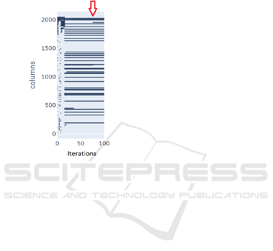
and remains stable. The figure shows 100 iterations

only due to the limited space.

Figure 7: Spatial Pooler soon after entering the stable state

become instable for some input patterns. After a few

iterations, the SP become stable again and it remains in the

stable state.

4 CONCLUSIONS

The Hierarchical Temporal Memory algorithm is

inspired by the neo-cortex and implements many

known features that have roots in neuro-sciences.

Nowadays many results show that the algorithm is

very flexible and can solve different kind of

problems. However, the reverse engineering of the

neo-cortex is still a complex and unsolved task. Many

design decisions in the algorithm base on assumptions

and work in progress. This paper focuses on the

instability issue of the HTM Spatial Pooler algorithm,

which has a task to memorize spatial patterns in an

unsupervised way. As discussed, the original Spatial

Pooler already integrates some sort of homeostatic

plasticity mechanism discovered in previous work in

neurosciences. However, the existing solution causes

instability in the learning process, which makes very

difficult to build applications. This work briefly

documented the named issue and offered the solution

by extending the existing SP algorithm with the new

component called Homeostatic Plasticity Controller.

The extended version of the SP is motivated by

finding in neurosciences, that documents the activity

of this mechanism during the development of the

species. Inspired with this finding the new

Homeostatic Plasticity Controller defines the

newborn stage of the Spatial Pooler. In this stage, the

SP stimulates the boosting of mini-columns and first

allows the instability in the learning process. After

the specified number of iterations, the HPC switches

off the boosting and waits for the SP to enter the

stable state. With this approach the SP converges to

the stable state and applications can be notified about

the state of the SP. This improves the quality of the

learning of the SP and enables the implementation of

more reliable solutions. Another work in progress in

this context is related to the design of the parallel

version of the HTM. The new HPC algorithm needs

to be validated for parallel implementation (Dobric,

Pech, Ghita and Wennekers, 2019).

REFERENCES

Davis, Graeme. (2006). Homeostatic Control of Neural

Activity - From Phenomenology to Molecular Design.

Annu. Rev. Neurosci. doi:10.1146

Davis, Graeme. (2013). Homeostatic Signaling and the

Stabilization of Neural Function. Neuron, 09.044.

Dobric. (2020). Implementation of Homeostatic Plasticity

Controller. Retrieved from GitHub - NeoCortexApi

repository: https://github.com/ddobric/neocortexapi/

blob/master/NeoCortexApi/NeoCortexApi/Homeostati

cPlasticityController.cs

Dobric, D. (2018). GitHub. Retrieved from NeoCortexAPI:

https://github.com/ddobric/neocortexapi

Dobric, Pech, Ghita, Wennekers. (2019). SCALING THE

HTM SPATIAL POOLER. International Journal of

Artificial Intelligence, 11(4).

Hawkins, Subtei. (2016). Why Neurons Have Thousands of

Synapses, a Theory of Sequence Memory in Neocortex.

Frontiers in neural circuts. doi:10.3389/

fncir.2016.00023

Hawkins, Subutai, & Cui. (2017). A Theory of How

Columns in the Neocortex Enable Learning the

Structure of the World. Frontiers in Neural Circuits,

11, 81-81. Retrieved 10 17, 2020, from

https://frontiersin.org/articles/10.3389/fncir.2017.0008

1/full

Maffei, Nelson, Turrigiano. (2004). Selective

reconfiguration of layer 4 visual cortical circuitry by

visual. Nature neuroscience, 1353-9.

Mountcastle. (1997). The columnar organization of the

neocortex. Journal of neurology, 120, 701-22.

Subutai, Hawkins. (2016). How do neurons operate on

sparse distributed representations? A mathematical

theory of sparsity, neurons and active dendrites.

ResearchGate.

Tien, Kerschensteiner. (2018). Homeostatic plasticity in

Improved HTM Spatial Pooler with Homeostatic Plasticity Control

105

neural development. ND - Neural Development, 13/9.

doi:10.1186

Turrigiano, Nelson. (2004). Homeostatic plasticity in the

developing nervous system. Nature Reviews

Neuroscience, 97–107.

Yuwei; Subutai; Hawkins. (2017). The HTM Spatial

Pooler, A Neocortical Algorithm for Online Sparse

Distributed Coding. Frontiers in computational

neurosciences, 11, 111.

APPENDIX

All experiments described in this paper are

implemented in C#/.NET Core 31. The Hierarchical

Temporal Memory framework with the Spatial Pooler

used in experiments is based on the open-source

project NeocortexApi. The source code and

documentation can be found at the GitHub (Dobric,

GitHub, 2018).

The experiment related to the stability of the

Spatial Pooleris implemented in a form of the

UnitTest inside of the Microsoft Unit Testing

framework integrated in Visual Studio. The test used

for the stability experiment is called

SpatialPooler_Stability_Experiment_3. It is

implementedin the source file SbStability.cs. This

code generatesthree output CSV files:-

ActiveColumns.csv,

-ActiveColumns-plotlyinput.csv and

-Oscilations.csv.

ActiveColumns files hold the same information in

a slightlydifferent format than ActiveColumns-

plotlyinput.csv. Bothfiles contain active columns

(SDR) for every trained digit in every iteration.

ActiveColumns-plotlyinput.csv can be used as the

input for the Python script to generate diagrams that

represent activecolumns shown in figure 6.

The script used go generate the diagram is called

draw_figure.py and can be found at the following

location:

/Python/ColumnActivityDiagram/draw_figure.py

Further information about running the script can

be foundin the Pyhton script

The file Oscilations.csv file is used to generate the

diagramshown in Figure 1. This diagram was

generated by Microsoft Excel.

ICPRAM 2021 - 10th International Conference on Pattern Recognition Applications and Methods

106