
Possibilities of using Neural Networks to Blood Flow Modelling
Katar
´
ına Buz
´
akov
´
a
1 a
, Katar
´
ına Bachrat
´
a
1 b
, Hynek Bachrat
´
y
1 c
and Michal Chovanec
2
1
Department of Software Technology, Faculty of Management Science and Informatics, University of
ˇ
Zilina,
ˇ
Zilina, Slovakia
2
Tachyum, s.r.o., Bratislava, Slovakia
Keywords:
Convolutional Neural Networks, Microfluidic Devices, Red Blood Cells Trajectory Prediction.
Abstract:
Computer simulation of the flow of blood or other fluid is beneficial to reduce the variety of costs necessary
for biological experiments in microfluidics. It turns out, that as biological experiments, even the simulations
have limitations. However, data from both types of experiments can be further processed by machine learning
methods in order to improve them and thus contribute to the optimization of microfluidic devices. This article
describes the possibilities of using neural networks to blood flow modelling. In this paper, we focus mainly
on the prediction of red blood cells movement. We propose other possibilities of using neural networks with
regard to the needs of further research in simulation modelling.
1 INTRODUCTION
Nowadays, the blood flow in microfluidic devices is
studied in many biological and medical researches,
see (Chen et al., 2012; Guo et al., 2017) for exam-
ple. The aim of the Cell in Fluid, Biomedical Mod-
eling & Computation Group is to optimize microflu-
idic devices to capture and sort cancer cells from other
solid components of blood. The reason is to use these
devices for early diagnosis of cancer from a blood
sample. The starting point of our research group’s
work a few years ago was that the design of microflu-
idic devices and the optimization of their performance
by real testing puts high demands on time, cost and
equipment. The solution was to create an extensive
simulation model in which experiments can be per-
formed in silico. For the description of the simulation
model see (Cimr
´
ak et al., 2012; Cimr
´
ak et al., 2014;
Cimr
´
ak and Jan
ˇ
cigov
´
a, 2018).
Current development of our work has resulted in
situations where the simulations are becoming too
complex and demanding in terms of time and com-
putational power. This complexity results in particu-
lar from the geometry and the size of the simulated
device, the number of modelled RBCs, the quantity
of watched and recorded measurements and also the
duration of the simulation. One simulation run often
several days or weeks. This is restrictive for repeating
a
https://orcid.org/0000-0001-7615-0038
b
https://orcid.org/0000-0002-5510-5585
c
https://orcid.org/0000-0003-1378-488X
or expanding simulation experiments with the same or
slightly altered parameters. On the other hand, each
of the simulations contains a huge amount of out-
put data, of which often only a small part is needed
to evaluate the specific phenomenon under investiga-
tion. From studies (Bachrat
´
a et al., 2017a; Bachrat
´
a
et al., 2017b; Bachrat
´
y et al., 2017; Bachrat
´
y et al.,
2018) turn out that these output data can be compre-
hensively described and characterized the course of
individual experiments using various statistical meth-
ods. We also used statistical methods to compare and
evaluate the quality of simulation experiments. Be-
cause we have large output data from simulations and
neural networks can find hidden features in the data,
this led us to the idea of complex processing of the
output data of simulation experiments using neural
networks. This should allow us to use them to ex-
tend and obtain further results without the need to per-
form new simulations. We do not use data from video
recordings of biological experiments because they do
not provide sufficiently large and accurate data. In
our research, we decided to use convolutional neural
networks because they can successfully capture the
spatial and temporal dependence in the image using
appropriate filters. In this case, the images represent
the locations of the cells in the channel in the individ-
ual time steps of the simulation.
This is also indicated by studies in other fields
using machine learning methods, where simulations
are significantly limited, see (Exl et al., 2019; Gusen-
bauer et al., 2020).
140
Buzáková, K., Bachratá, K., Bachratý, H. and Chovanec, M.
Possibilities of using Neural Networks to Blood Flow Modelling.
DOI: 10.5220/0010314101400147
In Proceedings of the 14th International Joint Conference on Biomedical Engineering Systems and Technologies (BIOSTEC 2021) - Volume 3: BIOINFORMATICS, pages 140-147
ISBN: 978-989-758-490-9
Copyright
c
2021 by SCITEPRESS – Science and Technology Publications, Lda. All rights reserved

1.1 Machine Learning for Blood Flow
Modelling
In this section, we introduce our results of using ma-
chine learning to simulate the blood flow. Since red
blood cells (RBCs) form a major part of haematocrit,
the correct modelling of their behaviour is decisive
in these simulations. The first results of machine
learning approach were presented in (Bachrat
´
y et al.,
2018). The foundation of this study is the use of ex-
tensive and detailed data outputs of simulations de-
scribing RBC trajectories in the examined channel.
These were used as a training and testing input for
learning algorithms that created radial basis function
network based on Kohonen’s self-organized maps. In
(Chovanec et al., 2019; Chovanec et al., 2019), con-
volutional neural networks (CNN) predict the RBC
center velocity vector in the channel. This allow us
to:
• virtually extend or artificially create new RBC tra-
jectories,
• estimate the impact of RBC motion on cancer cell
behaviour at at all examined points in the channel
points in the channel,
• improve RBC tracking when processing videos of
real experiments.
These papers describe ways of CNN learning, the ac-
curacy of trajectory predictions and their dependence
on neural network architecture, type of input parame-
ters and methodology of verification and selection of
appropriate neural network experiments.
1.2 Prediction of Red Blood Cells
Trajectory
Here we describe how neural networks predict red
blood cells movement. In (Chovanec et al., 2019)
we created a framework for predicting RBCs trajec-
tories in microfluidic channels using CNN. (In what
follows we will call it the prediction model and neu-
ral networks (NN) experiments as prediction exper-
iments.) In this model, the network learns to predict
the velocity vector of a cell’s center from the temporal
sequence of its previous positions. This information
comes from the simulation outputs. More information
about simulation outputs and their processing for the
model are in the work (Chovanec et al., 2019). The
velocity of the cell in the microchannel is affected by
various factors, for example the previous movement
of the cell, the motion of other particles, the topol-
ogy of the channel, the speed of the liquid which is
different in the channel slits than in the areas free
from obstacles. For the trajectory prediction itself,
we determine cells positions from their predicted ve-
locities. By repeating this procedure, predicted posi-
tions are determined from predicted velocities for all
time steps. Finally, we obtain the predicted trajecto-
ries from the initial trajectories of all modelled cells.
(Figure 1). Note that the obtained RBC trajectory is
a set of discrete points, which represents positions of
the cell’s center in all time steps of the prediction ex-
periment.
2 DATASETS
Datasets for the prediction experiments come from
simulations. As the output of a simulation experi-
ment, we obtain miscellaneous characteristics about
cells. From these data, we extract the coordinates
of the centers of the cells and their velocity vectors.
Then we use this information as an entry for the pre-
diction experiment.
For a given prediction experiment, we use data
from simulations, which vary in the initial seeding
of RBCs. Hence, the cell trajectories in these ex-
periments are different from each other. However,
there should be similarities in the trajectories, since
all other setups of these simulations are the same.
It includes elastic parameters of cells, fluid parame-
ters and geometry of microchannel. These data are
divided to training and testing sets for neural net-
work. The training set consist of extracted data from
one simulation experiment and data for the testing set
comes from the second simulation experiment output.
2.1 Simulation Experiment Designs
Simulation experiments use Open-source software
ESPResSo (Arnold et al., 2013). The fluid is
modelled using the Lattice-Boltzmann method, see
(Ahlrichs and D
¨
unweg, 1998). RBCs and other
elastic objects are immersed in the fluid (Cimr
´
ak
et al., 2014).
For prediction experiments, we use simulations of
blood flow in two microfluidic devices with different
topology described below. The RBC model is the tri-
angulation of its surface. Both simulations use RBC
model with 374 nodes and the size of RBC in a re-
laxed state is 7, 8µm × 7, 8µm × 2, 56µm. The direc-
tion of the blood flow is from left to right along the
horizontal x-axis. The channels are periodic (in this
direction) in a sense that the cell which leaves the sim-
ulation channel at one end reenters the channel on the
other end.
Possibilities of using Neural Networks to Blood Flow Modelling
141
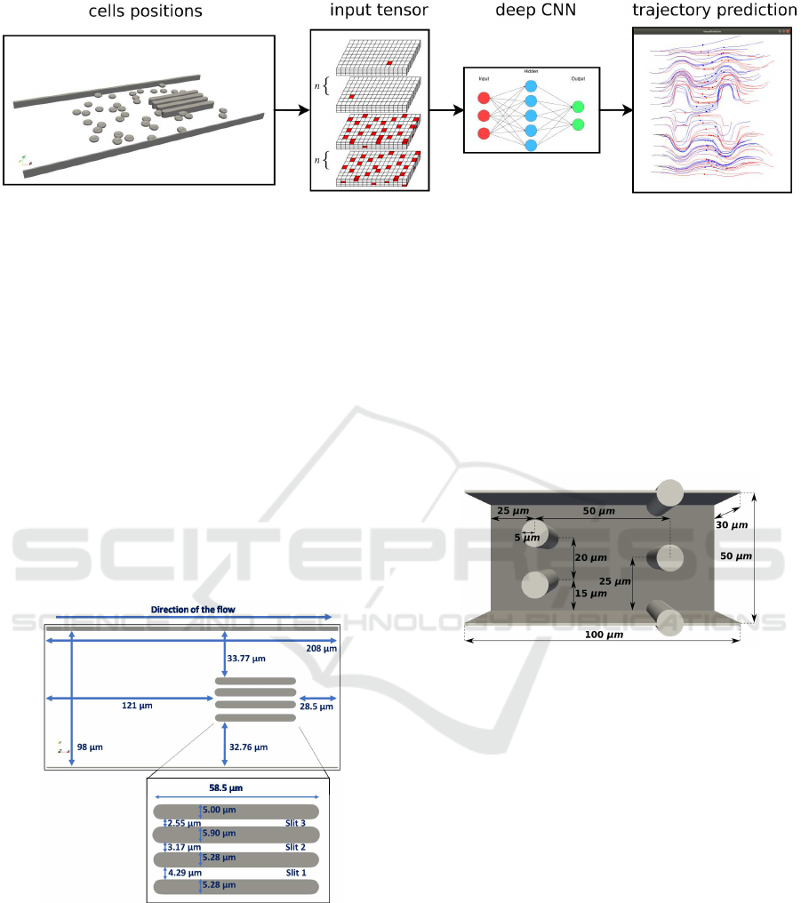
Figure 1: Red blood cells trajectory prediction using CNN.
2.1.1 Channel with Narrow Slits
The simulation of this channel is based on the labora-
tory experiment described in (Tsai et al., 2016). This
paper studies the correlation between RBC velocity
and its deformation in narrowings of the microfluidic
channel formed by obstacles. The internal dimensions
of the simulation channel are 208µm×98µm ×3.5µm.
There are 4 longitudinal obstacles in the channel, see
Figure 2. To fit the haematocrit used in the laboratory
experiment, the number of blood cells in the simula-
tion experiment is 38. At the beginning of the sim-
ulation, all cells were in the left part of the channel.
A more detailed description of the simulation can be
found in (Koval
ˇ
c
´
ıkov
´
a et al., 2019). We will refer to
the dataset and the channel from this simulation as
dataset A and simulation channel A.
Figure 2: Simulation channel A with narrow slits.
2.1.2 Channel with Cylindrical Obstacles
Simulations of the blood flow in the channel with
cylindrical obstacles were an important tool to design
and test most of the RBC characteristics used in the
simulation model, for example the absolute cell ve-
locity, the position, the slope and the rotation of RBC
or a periodic behaviour in the channel, see (Bachrat
´
a
et al., 2017b; Bachrat
´
y et al., 2017; Bachrat
´
a et al.,
2017a). The channel is shown in Figure 3. It is a
cuboid of size 100µm × 50µm × 30µm and it contains
5 cylindrical obstacles with a diameter of 5µm. An
element of each cylinder is parallel to the z-axis and
the height of each cylinder is equal to the height of
the simulation channel. The amount of RBCs in ex-
periments is 100. The initial seeding of the cells is
random in the whole space of the simulation channel.
We will refer to the dataset and the channel from this
simulation as dataset B and simulation channel B.
Figure 3: Simulation channel B with cylindrical obstacles.
The calibration of elastic coefficients of the cell’s
model was made by stretching experiment. The de-
tailed explanation of the calibrating process is ex-
plained in (T
´
othov
´
a et al., 2015). The obtained elas-
tic parameters for simulation models are summarised
in Table 1.Another type of parameters which had to
be set separately for each cell model are the interac-
tion parameters between cells. These parameters pre-
vent cell collisions. They are summarised in Table
2.The numerical parameters of simulation liquid are
depicted in Table 3.
3 NEURAL NETWORK MODEL
In this section we first introduce neural network input.
Then we describe the networks architectures, hyper-
parameters that are used and other details.
BIOINFORMATICS 2021 - 12th International Conference on Bioinformatics Models, Methods and Algorithms
142
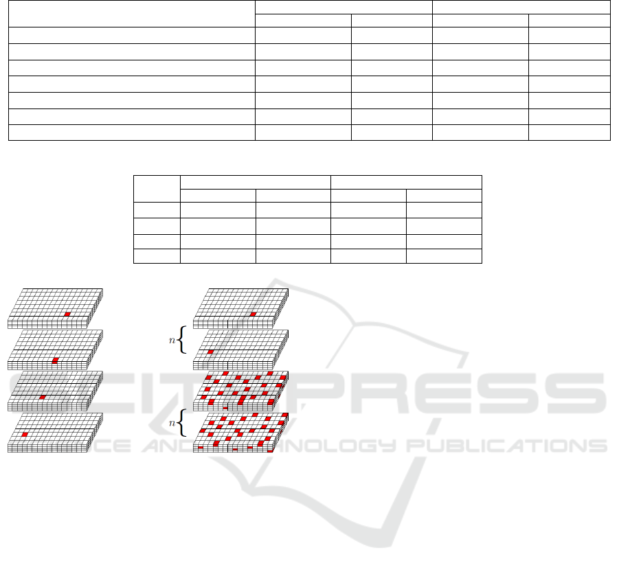
Table 1: Elastic parameters of the cell model used in simulation experiments, established by simulation of stretching experi-
ment.
simulation A simulation B
LB units SI units LB units SI units
Radius 3.91Lm 3.91
∗
10
−6
m 3.91Lm 3.91
∗
10
−6
m
Stretching coefficient k
s
6
∗
10
−3
LN/Lm 6
∗
10
−6
N/m 5
∗
10
−3
LN/Lm 5
∗
10
−6
N/m
Bending coefficient k
b
8
∗
10
−3
LNLm 8
∗
10
−18
Nm 3
∗
10
−3
LNLm 3
∗
10
−18
Nm
Coefficient of local area conservation k
al
1
∗
10
−3
LN/Lm 1
∗
10
−6
N/m 2
∗
10
−2
LN/Lm 2
∗
10
−4
N/m
Coefficient of global area conservation k
ag
0.9LN/Lm 9
∗
10
−4
N/m 0.7LN/Lm 7
∗
10
−4
N/m
Coefficient of volume conservation k
v
0.5LN/Lm
2
5
∗
10
2
N/m
2
0.9LN/Lm
2
9
∗
10
2
N/m
2
Membrane viscosity 0Lm
2
/Ls 0m
2
/s 0Lm
2
/Ls 0m
2
/s
Table 2: Parameters of inter-cellular interactions.
simulation A simulation B
LB units SI units LB units SI units
a 2
∗
10
−3
(−) 2
∗
10
−3
(−) 1
∗
10
−3
(−) 1
∗
10
−3
(−)
n 1.5Lm 1.5
∗
10
−6
m 1.2Lm 1.2
∗
10
−6
m
cutoff 0.4(−) 0.4(−) 0.5(−) 0.5(−)
offset 0(−) 0(−) 0(−) 0(−)
Figure 4: Input tensor based on spatial discretization of the
channel.
3.1 CNN Input
Inputs to the neural network are tensors. They are
based on the discretization of the simulation channel
to a three-dimensional rectangular network in which
the position and movement of cells is described by
their occupation evolving over time (Figure 4). For
more detailed description of the input see (Chovanec
et al., 2019; Chovanec et al., 2019). In (Chovanec
et al., 2019) we compared this input format with an-
other input format based on the numerical expression
of the cell’s center positions. For the input based on
discretization, the maximum error of the experiments
performed was 3.26%. For the other input type, the
error of the performed experiments was in the range
of approximately 10% to 40%.
In (Chovanec et al., 2019) we tested the impact of
various modifications of CNN input on the accuracy
of the prediction experiment. In both of these stud-
ies, we used the dataset A from the simulations of the
channel with narrow slits.
3.2 Networks Architectures
In prediction experiments, we use 3 different CNN
architectures net 0,net 1 and net 2 for both dataset A
and dataset B. We chose these architectures based on
the accuracy of NN experiments in our previous stud-
ies (Chovanec et al., 2019; Chovanec et al., 2019) and
also with regard to the latest improvements in the field
of neural networks. In these models we use the activa-
tion function ELU (Clevert et al., 2015). For dataset
B, we also use net 6, which we used for dataset A in
(Chovanec et al., 2019). Networks architectures are
shown in Figure 4. In networks net 0 and net 1, there
are alternating convolution layers with max pooling
layers. At the end, there are 2 fully connected layers
with 256 and 3 neurons, respectively. Network net 1
differs from network net 0 by adding spatial attention
layers (Vaswani et al., 2017). In network net 2, com-
pared to net 1, 4 dense blocks (Huang et al., 2017) are
used instead of 3 × 3 convolution kernels.
3.2.1 Hyperparameters
All CNN architectures have the following hyperpa-
rameters: weights are initialized using xavier (Glorot
and Bengio, 2010); the bias is set to 0; minibatch size
is 32 (Li et al., 2014).
Regularization parameters are: dropout = 2 · 10
−2
;
L
1
= L
2
= 1 · 10
−6
. We also use feature pooling with
1 × 1 kernels to prevent overfitting.
Possibilities of using Neural Networks to Blood Flow Modelling
143
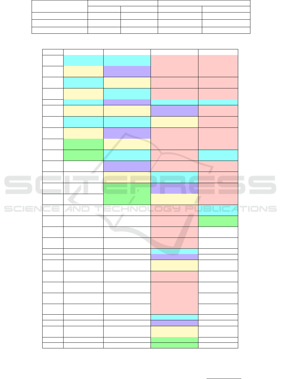
Table 3: The numerical parameters of simulation liquid.
simulation A simulation B
LB units SI units LB units SI units
Density 1Lkg/Lm
3
1
∗
10
3
kg/m
3
1.025Lkg/Lm
3
1.025
∗
10
3
kg/m
3
Kinematic viscosity 1Lm
2
/Ls 1
∗
10
−6
m
2
/s 1.3Lm
2
/Ls 1.3
∗
10
−6
m
2
/s
Friction coeff. 1.15(−) 1.15(−) 1.41(−) 1.41(−)
Table 4: Networks architectures.
layer net 0 net 1 net 2 net 6
0
conv 3x3x32 conv 3x3x32
dense conv
3x3x8
dense conv
3x3x8
1
max pooling
2x2x1
spatial attention
dense conv
3x3x8
dense conv
3x3x8
2
conv 3x3x32
max pooling
2x2x1
dense conv
3x3x8
dense conv
3x3x8
3
max pooling
2x2x1
conv 3x3x32
dense conv
3x3x8
dense conv
3x3x8
4
conv 3x3x64
spatial attention
conv 1x1x32 conv 1x1x16
5
max pooling
2x2x1
max pooling
2x2x1
spatial attention
dense conv
3x3x8
6
conv 3x3x64 conv 3x3x64
max pooling
2x2x1
dense conv
3x3x8
7
max pooling
2x2x1
spatial attention
dense conv
3x3x8
dense conv
3x3x8
8 fc 256
max pooling
2x2x1
dense conv
3x3x8
dense conv
3x3x8
9 fc 3
conv 3x3x64
dense conv
3x3x8
conv 1x1x16
10
spatial attention
dense conv
3x3x8
dense conv
3x3x8
11
max pooling
2x2x1
conv 1x1x32
dense conv
3x3x8
12 fc 256
spatial attention
dense conv
3x3x8
13 fc 3
max pooling
2x2x1
dense conv
3x3x8
14
dense conv
3x3x8
conv 1x1x32
15
dense conv
3x3x8
fc 3
16
dense conv
3x3x8
17
dense conv
3x3x8
18 conv 1x1x64
19
spatial attention
20
max pooling
2x2x1
21
dense conv
3x3x8
22
dense conv
3x3x8
23
dense conv
3x3x8
24
dense conv
3x3x8
25 conv 1x1x64
26
spatial attention
27
max pooling
2x2x1
28 fc 256
29 fc 3
3.3 Networks Training
In all prediction experiments, we use training algo-
rithm ADAM (Kingma and Ba, 2015) and learning
rate is set to 2 · 10
−4
. We minimalize the loss func-
tion:
MSE =
∑
n
i=1
(y
i
− ˆy
i
)
2
n
,
BIOINFORMATICS 2021 - 12th International Conference on Bioinformatics Models, Methods and Algorithms
144

where y
i
are target values, ˆy
i
are predicted values and
n is the dataset size.
For both datasets and for the nets net 0, net 1 and
net 2, the networks did not trained enough. We sup-
pose, it is due to the fully connected layer with 256
neurons. For net 6 and for dataset B, the value of
loss function was significantly lower at the end of the
training. Note, that we used this network and net-
works with similar architectures in (Chovanec et al.,
2019). Thus, we suspected good training results for
this network. Moreover, there is bigger decrease of
loss function from the beginning to the end of the
training than for the dataset A trained on net 6 in
(Chovanec et al., 2019).
4 DATASET DAMAGING
In this section, we propose a method of using neural
networks to detect and eliminate possible errors and
inaccuracies of simulation experiments. During our
simulation experiments, we encountered inaccuracies
in the simulation outputs several times. These errors
may be due to the improper calibration of the simula-
tion parameters, numerical errors caused by computa-
tional algorithms or measurement errors with respect
to data obtained by processing laboratory experiment
records. For example, in the simulation model, inac-
curacies are encountered in the calculation of veloc-
ity of cells center and nodes. Figure 5 shows graphs
comparing the y- and z-coordinates of the cell’s center
velocity obtained from the simulation, and the same
coordinates computed from the cell’s center positions
(determined by the simulation). This simulation was
used in (Bachrat
´
y et al., 2018). This could serve as
a tool to correct the simulation experiments, since to
correct the simulation by using a prediction experi-
ments is faster then to run the simulation again with
slightly altered setup.
Our aim is to find out at what extent of the dam-
age we can still predict the movement of blood cells
with sufficient accuracy. To do this we intentionally
damage a part of the training data. The data damage
can be described using three parameters:
1. type,
2. percentage,
3. data corruption level.
The parameter type says what kind of data is dam-
aged. In our prediction experiments, it can be cell’s
center positions or velocities. The second parameter
determines the percentage of damaged data. Finally,
data corruption level is the degree of inaccuracy of a
damaged value compared to the actual value.
For the percentage p% of the cell’s positions
damage with the d% data corruption level, we
randomly damage p% of positions as follows:
c
damaged
= (1 − 0.01 · d)c + 0.01 · d · rand(−1,1),
where c corresponds to the value of individual
coordinates x,y and z normalized to the interval h0,1i
as is common in neural networks, and rand(−1,1) is
a random value from the range (−1,1).
Damaged value in coordinate c is then
c
damaged
=
c
damaged
, if c
damaged
∈ (0,1),
0, if c
damaged
< 0,
1, if c
damaged
> 1.
5 PREDICTION BASED ON
LOCAL AREA INFORMATION
The study (Chovanec et al., 2019) shows that the ac-
curacy of the prediction experiment depends on the
input data format. A format based on the discretiza-
tion of the channel to a three-dimensional rectangular
network (see 3.1) seems to be clearly more appropri-
ate.
The discretization of the channel affects the size
of the input tensor for the neural network. It is lim-
ited in the z-axis by the depth of the neural network.
Due to the computational complexity, we can only
use discretizations smaller than 9 in this direction,
which is not sufficient for deeper microfluidic chan-
nels. Instead, we can only look at the close local
area of the monitored RBC, and use a finer discretiza-
tion of the situation there (see Figure 6, the cell of
an interest is in the red rectangle, and for this rectan-
gle we use a finer discretization). This discretization
is three-dimensional, captures the position of the cell
of an interest and other objects in the neighborhood,
that is, other cells, channel walls and obstacles. It
describes positions of cells more precisely, hence it
could be used to predict other characteristics of cells
movement, such as the rotation and slope. One of
the most important purposes of this local prediction
model should be the prediction of cells movement in
channels with different topology. It means that topol-
ogy of a channel used for training is different from the
topology of a simulation channel used in testing. This
is of great interest for simulating process because sim-
ulations of large channels are computationally very
difficult or even impossible to run. An interesting
question is if a network trained on these local data will
be able to predict the RBC behaviour globally across
the channel with sufficient accuracy.
Possibilities of using Neural Networks to Blood Flow Modelling
145
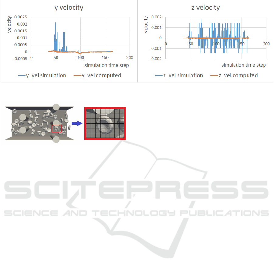
Figure 5: Cell center velocity at y and z coordinates. The blue curve shows the speed calculated by the simulation. The orange
line represents the speed computed from the cell center positions.
Figure 6: Discretization of local area of the simulation
channel.
6 CONCLUSIONS
This paper presents the possibilities of the use of neu-
ral networks to optimize simulation and biological ex-
periments of blood flow in microfluidic devices. It
deals mainly with the prediction of the trajectory of
red blood cells, which can significantly help in the
tracing of red blood cells from video recordings of
real experiments. This is also useful in simulating
blood flow where simulations are limited by compu-
tational complexity. Furthermore, we point out the
ways of improving prediction experiments and pro-
pose their further use. This would be especially useful
for predicting the movement of blood cells in devices,
for which, due to their topology, current simulation
experiments cannot be performed. Further, this can
be used to detect possible inaccuracies of simulation
outputs, and to investigate other characteristics of red
blood cells needed for the proper simulation model.
ACKNOWLEDGEMENTS
This work was supported by the Ministry of Educa-
tion, Science, Research and Sport of the Slovak Re-
public (contract No. VEGA 1/0643/17) and by Op-
erational Program ”Integrated Infrastructure” of the
project ”Integrated strategy in the development of per-
sonalized medicine of selected malignant tumor dis-
eases and its impact on life quality”, ITMS code:
313011V446, co-financed by resources of European
Regional Development Fund.
REFERENCES
Ahlrichs, P. and D
¨
unweg, B. (1998). Lattice-boltzmann
simulation of polymer-solvent systems. International
Journal of Modern Physics C (IJMPC), 09(08):1429–
1438.
Arnold, A., Lenz, O., Kesselheim, S., Weeber, R., Fahren-
berger, F., Roehm, D., Kosovan, P., and Holm, C.
(2013). Espresso 3.1 — molecular dynamics software
for coarse-grained models. In Meshfree Methods for
Partial Differential Equations VI, volume 89.
Bachrat
´
a, K., Bachrat
´
y, H., and Koval
ˇ
c
´
ıkov
´
a, K. (2017a).
The sensitivity of the statistical characteristics to the
selected parameters of the simulation model in the red
blood cell flow simulations. In 2017 International
Conference on Information and Digital Technologies
(IDT), pages 344–349.
Bachrat
´
a, K., Bachrat
´
y, H., and Slav
´
ık, M. (2017b). Statis-
tics for comparison of simulations and experiments
of flow of blood cells. EPJ Web of Conferences,
143:02002.
Bachrat
´
y, H., Bachrat
´
a, K., Chovanec, M., Kaj
´
anek, F.,
Smie
ˇ
skov
´
a, M., and Slav
´
ık, M. (2018). Simulation
of Blood Flow in Microfluidic Devices for Analysing
of Video from Real Experiments, pages 279–289.
Springer International Publishing.
Bachrat
´
y, H., Koval
ˇ
c
´
ıkov
´
a, K., Bachrat
´
a, K., and Slav
´
ık, M.
(2017). Methods of exploring the red blood cells ro-
tation during the simulations in devices with periodic
topology. In 2017 International Conference on Infor-
mation and Digital Technologies (IDT), pages 36–46.
IEEE.
Chen, J., Li, J., and Sun, Y. (2012). Microfluidic approaches
for cancer cell detection, characterization, and separa-
tion. Lab on a Chip, 12(10):1753–1767.
Chovanec, M., Bachrat
´
y, H., Jasen
ˇ
c
´
akov
´
a, K., and
Bachrat
´
a, K. (2019). Influence of cnn input modifica-
tion for red blood cells trajectory prediction in blood
BIOINFORMATICS 2021 - 12th International Conference on Bioinformatics Models, Methods and Algorithms
146

flow. In 2019 IEEE 15th International Scientific Con-
ference on Informatics, pages 469–476.
Chovanec, M., Bachrat
´
y, H., Jasen
ˇ
c
´
akov
´
a, K., and
Bachrat
´
a, K. (2019). Convolutional neural networks
for red blood cell trajectory prediction in simulation
of blood flow. In International Work-Conference on
Bioinformatics and Biomedical Engineering, pages
284–296. Springer.
Cimr
´
ak, I., Gusenbauer, M., and Jan
ˇ
cigov
´
a, I. (2014).
An espresso implementation of elastic objects im-
mersed in a fluid. Computer Physics Communications,
185(3):900–907.
Cimr
´
ak, I., Gusenbauer, M., and Schrefl, T. (2012). Mod-
elling and simulation of processes in microfluidic
devices for biomedical applications. Computers &
Mathematics with Applications, 64(3):278–288.
Cimr
´
ak, I. and Jan
ˇ
cigov
´
a, I. (2018). Computational Blood
Cell Mechanics: Road Towards Models and Biomedi-
cal Applications. CRC Press.
Clevert, D.-A., Unterthiner, T., and Hochreiter, S. (2015).
Fast and accurate deep network learning by exponen-
tial linear units (elus). Under Review of ICLR2016
(1997).
Exl, L., Mauser, N., Schrefl, T., and Suess, D. (2019).
Learning time-stepping by nonlinear dimensionality
reduction to predict magnetization dynamics.
Glorot, X. and Bengio, Y. (2010). Understanding the dif-
ficulty of training deep feedforward neural networks.
Journal of Machine Learning Research - Proceedings
Track, 9:249–256.
Guo, Q., Duffy, S., Matthews, K., Islamzada, E., and Ma,
H. (2017). Deformability based cell sorting using mi-
crofluidic ratchets enabling phenotypic separation of
leukocytes directly from whole blood. Scientific Re-
ports, 7.
Gusenbauer, M., Oezelt, H., Fischbacher, J., Kovacs, A.,
Zhao, P., Woodcock, T., and Schrefl, T. (2020). Ex-
tracting local nucleation fields in permanent magnets
using machine learning. npj Computational Materi-
als, 6:1–10.
Huang, G., Liu, Z., Van Der Maaten, L., and Weinberger,
K. Q. (2017). Densely connected convolutional net-
works. In 2017 IEEE Conference on Computer Vision
and Pattern Recognition (CVPR), pages 2261–2269.
Kingma, D. P. and Ba, J. (2015). Adam: A method for
stochastic optimization. In Bengio, Y. and LeCun,
Y., editors, 3rd International Conference on Learn-
ing Representations, ICLR 2015, San Diego, CA, USA,
May 7-9, 2015, Conference Track Proceedings.
Koval
ˇ
c
´
ıkov
´
a, K., Cimr
´
ak, I., Bachrat
´
a, K., and Bachrat
´
y, H.
(2019). Comparison of Numerical and Laboratory Ex-
periment Examining Deformation of Red Blood Cell,
pages 75–86. Springer International Publishing.
Li, M., Zhang, T., Chen, Y., and Smola, A. J. (2014). Ef-
ficient mini-batch training for stochastic optimization.
In KDD, pages 661–670.
T
´
othov
´
a, R., Jan
ˇ
cigov
´
a, I., and Bu
ˇ
s
´
ık, M. (2015). Calibra-
tion of elastic coefficients for spring-network model
of red blood cell. In 2015 International Conference
on Information and Digital Technologies, pages 376–
380. IEEE.
Tsai, C.-H., Tanaka, J., Kaneko, M., Horade, M., Ito, H.,
Taniguchi, T., Ohtani, T., and Sakata, Y. (2016). An
on-chip rbc deformability checker significantly im-
proves velocity-deformation correlation. Microma-
chines, 7.
Vaswani, A., Shazeer, N., Parmar, N., Uszkoreit, J., Jones,
L., Gomez, A. N., Kaiser, L. u., and Polosukhin, I.
(2017). Attention is all you need. In Guyon, I.,
Luxburg, U. V., Bengio, S., Wallach, H., Fergus, R.,
Vishwanathan, S., and Garnett, R., editors, Advances
in Neural Information Processing Systems 30, pages
5998–6008. Curran Associates, Inc.
Possibilities of using Neural Networks to Blood Flow Modelling
147
