Analysing Adversarial Examples for Deep Learning

Jason Jung, Naveed Akhtar and Ghulam Mubashar Hassan

Department of Computer Science & Software Engineering, The University of Western Australia, Australia

Keywords: Adversarial Examples, Adversarial Attacks, Imagenet, Neural Networks, Image Classifiers.

Abstract: The aim of this work is to investigate adversarial examples and look for commonalities and disparities

between different adversarial attacks and attacked classifier model behaviours. The research focuses on

untargeted, gradient-based attacks. The experiment uses 16 attacks on 4 models and 1000 images. This

resulted in 64,000 adversarial examples. The resulting classification predictions of the adversarial examples

(adversarial labels) are analysed. It is found that light-weight neural network classifiers are more suspectable

to attacks compared to the models with a larger or more complex architecture. It is also observed that similar

adversarial attacks against a light-weight model often result in the same adversarial label. Moreover, the

attacked models have more influence over the resulting adversarial label as compared to the adversarial attack

algorithm itself. These finding are helpful in understanding the intriguing vulnerability of deep learning to

adversarial examples.

1 INTRODUCTION

Image classification with deep neural networks

performs remarkably well. A model can be trained by

feeding it thousands of images, resulting in the ability

to accurately classify even the breeds of a dog.

However, these trained models can easily be deceived

by adversarial attacks (Akhtar & Mian, 2018). A well

calculated imperceptible perturbation can cause these

models to completely misclassify an image. The

image plus perturbation is known as an ‘adversarial

example’. An adversarial example which may appear

as a cat to the human eye may be classified as a dog

or even something entirely different, such as a tree by

the network. Since the discovery of these adversarial

attacks, there has been continued research into

finding ways to make the models more robust against

these attacks. A kind of arms race has taken place to

find stronger attacks and stronger defences (Akhtar &

Mian, 2018).

There has been a focus on developing stronger

attacks, however there is a lack of ‘analysis’ for these

attacks and for deep neural network classifier models.

The aim of this work is to address this, and gain

insights into the behaviour of models under different

attacks and analysing their mutual relations. The

focus is on gradient-based untargeted attacks.

2 RELATED WORKS & ATTACKS

A comprehensive survey of adversarial attacks for

deep learning in computer vision was written in early

2018 (Akhtar & Mian, 2018). The survey serves as a

comprehensive introduction into adversarial attacks

for interested readers.

Adversarial examples were first discovered by

Szegedy, et al., 2014. The following problem was

defined: find the smallest perturbation such that,

1. The resulting adversarial example (input image +

perturbation) is misclassified as a specific

targeted label.

2. The adversarial example’s pixel values remain

within the pixel bounds of the original input

image.

Because of the non-trivial task of solving the above,

a box-constrained Limited memory Broyden-

Fletcher-Goldfarb-Shanno (L-BFGS) algorithm was

used to find an approximate solution (Szegedy, et al.,

2014). The resulting attack is referred to as the L-

BFGS attack and was the first adversarial attack.

In 2015, Goodfellow et al. proposed the idea that

the underlying cause of adversarial examples was the

linearity of neural networks. This idea led to the Fast

Gradient Sign Method (FGSM). To calculate the

perturbation for this attack, take the sign of the

Jung, J., Akhtar, N. and Hassan, G.

Analysing Adversarial Examples for Deep Learning.

DOI: 10.5220/0010313705850592

In Proceedings of the 16th International Joint Conference on Computer Vision, Imaging and Computer Graphics Theory and Applications (VISIGRAPP 2021) - Volume 5: VISAPP, pages

585-592

ISBN: 978-989-758-488-6

585

gradient of the cost function with respect to the input

image (Goodfellow, Shlens, & Szegedy, 2015).

The Basic Iterative Method (BIM) is an extension

of the FGSM. For this attack, the FGSM is repeated

multiple times using a small step-size. After each

iteration, the result is clipped to ensure the

perturbation is within the 𝜖 -neighbourhood of the

original image. These improvements allowed the

BIM to be a stronger attack with smaller perturbations

(Kurakin, Goodfellow, & Bengio, 2017).

Madry et al. proposed the strongest attack

utilizing the local first order information about the

network, the Projected Gradient Attack (PGD). The

attack works similarly to BIM however the PGD is

restarted from many random points in the l-inf ball to

better understand the loss landscape. (Madry,

Makelov, Schmidt, Tsipras, & Vladu, 2019).

The PGD was found to be inefficient in the l-1

case, so the Sparse l-1 Descent attack (SLIDE) was

proposed. For the l-1 norm, the PGD updates a single

index of the perturbation at a time. The SLIDE uses a

pre-set percentile, then updates multiple indices with

the steepest descent directions in this percentile. The

result is then normalised to the unit l-1 norm (Tramèr

& Boneh, 2019).

DeepFool is another iterative gradient based

attack (Moosavi-Dezfooli, Fawzi, & Frossard, 2016).

This attack algorithm tries to approximate

classification regions (the regions corresponding to

different labels) and hyperplanes at the boundaries of

these regions. From the current image, it takes the

projection to the closest hyperplane. This projection

is used as the perturbation. These steps are repeated

until the classification changes (i.e. an adversarial

example is found).

The Decoupled Direction and Norm Attack

(DDN) was proposed as an improvement over the

very popular Carlini & Wagner (C&W) attack and

DeepFool (Rony, et al., 2019). The iterative portion

of the algorithm starts with clean image 𝒙



and steps

in the direction of the gradient of the loss function (g).

Depending on whether the result 𝒙



𝑔 is

adversarial or not, a separate 𝜖



sphere around 𝒙 will

have its radius decreased or increased. The 𝒙



𝑔

will then be projected onto the new sphere and the

resulting projected point will be 𝒙



, to be used for

the next iteration.

The Brendel & Bethge Attack is a combination of

a boundary attack and gradient attack (Brendel,

Rauber, Kümmerer, Ustyuzhaninov, & Bethge,

2019). The attack works by starting from an

adversarial sample point far away from the clean

input. Then it estimates the local geometry of the

boundary between the adversarial and non-

adversarial regions and follows the adversarial

boundary towards the clean input. It attempts to

minimize the distance to the clean input while staying

on the adversarial boundary.

Although there has been much research into

various areas surrounding adversarial attacks, the

main focus has been on creating stronger attacks and

more robust models. The most common dataset used

has been MNIST and CIFAR10. These contain

smaller images (10x10, 32x32) which require simpler

models and only include a small number of classes.

This project explores adversarial attacks with the

much larger Imagenet dataset which involves larger

images and 1000 classes.

Attack Success Rates (ASR) and perturbation size

are common metrics used to compare attacks. Aside

from this, there is little research on how these attack

algorithms and models may be related. By

investigating the resulting labels of many adversarial

examples for various attacks and models, this

research project aims to identify some possible

relations, commonalities and disparities between the

attacks and models.

3 EXPERIMENTAL DESIGN

For clarity, the setup of the main experiment is kept

simple. Run 16 adversarial attacks against 4 deep

neural network models with 1000 images. This

resulted in 64,000 adversarial examples. The top

classification predictions (or labels) of the resulting

adversarial examples were recorded. In addition, the

confidences of these predictions, as well as the

perturbations, were recorded. This data was then

analyzed to gain insight into these attacks and models.

The following analysis was performed:

- Calculate the Attack Success Rates (ASRs) of the

different attack + model combinations. The ASR

is a fraction of adversarial attacks which

successfully cause misclassification. The aim is

to look for patterns for attacks and/or models.

- Evaluate how frequent the most commonly

appearing label occurred. The aim is to analyze

the major influencer on the resulting adversarial

labels.

- See how the labels/predictions of the clean image

may transform to become the top prediction of

the adversarial example.

- Compare the adversarial labels of the attacks.

Attacks which resulted in similar adversarial

labels could be considered as being similar and

vice versa.

VISAPP 2021 - 16th International Conference on Computer Vision Theory and Applications

586

3.1 Attacks

Gradient-based, untargeted attacks were chosen as the

adversarial attacks for this experiment. Gradient-

based attacks were used because of their simplicity

and variety. These attacks use the gradient of the cost

function w.r.t. the input to calculate the perturbation.

Targeted attacks aim to create an adversarial example

which is incorrectly classified as a specified class or

label (the target). Untargeted attacks do not care about

the resulting label of the adversarial example. They

simply minimize the chance of the correct label being

predicted. This work looks to analyze the resulting

labels of these untargeted attacks. The attacks shown

in Table 1 were used.

Table 1: Attack acronyms.

Acron

m Attac

PGD Pro

ected Gradient Descent

FGM

Fast Gradient Method – a generalized

version of FGM

BIM Basic Iterative Metho

SLIDE S

arse l-1 Descent

DF DeepFool

DDN Decou

led Direction and Nor

BBA Brendel and Beth

e Attac

These attacks can also be divided into Fixed

Epsilon Attacks (PGD, FGM, BIM, SLIDE) and

Minimization Attacks (DF, DDN, BBA). For Fixed

Epsilon Attacks, the epsilon or maximum

perturbation allowance is set before running the

attack. Minimization Attacks aim to minimize size

over the preset number of iterations.

Different perturbation l

norm versions of these

attacks were used. All 16 attacks can be seen in Table

2. The l

inf

norm is the maximum value of any element

of the perturbation. The l

norm is the sum of the

absolute values. The l

norm is the Euclidean norm

(square root of the sum of squares of the elements).

The perturbations for the attacks are restricted by

these norms.

Table 2: All adversarial attacks used in the main

experiment.

l-inf l-1 l-2

PGD PGD PGD

FGM FGM FGM

BIM BIM BIM

SLIDE

DDN

BBA BBA BBA

3.2 Models

Four deep neural network classifier models were

used: vgg16, resnet50, inception_v3 and mobilenet.

These models were chosen for their popularity,

availability and differences to one another. Vgg16 is

a deep network with its main feature being the many

convolutional layers. Resnet50 similarly consists of

many convolutional layers, however it is a residual

network, meaning it utilizes skip connections to

connect layers using shortcuts. Inception_v3 is a

complex network, using techniques such as

factorizing layers into smaller convolutions to reduce

the number of parameters and thus increase the

efficiency of the network. Mobilenet is an efficient,

light-weight network designed for mobile and

embedded vision applications.

3.3 Images

1000 images were used for this experiment. These

images were taken from the Imagenet database.

Specifically, from the ILSVRC2012 validation set.

From a set of images which were classified correctly

by all 4 experiment models, 1000 images were

randomly chosen.

3.4 Foolbox

The python library Foolbox was used to run the attack

algorithms and generate perturbations. Foolbox is a

popular library used for adversarial attacks against

machine learning models and benchmarking the

robustness of models against adversarial attacks

(Rauber, Zimmermann, Bethge, & Brendel, 2020).

The popularity, variety of attacks and fast

performance of the library made it a suitable choice

for this project.

3.5 Parameters

The parameters in Table 3 were used for this

experiment. The parameters were chosen mainly

based on previous works. The number of steps was

chosen based on experiment 2 results and with

consideration of the amount of time required to run

all the attacks. It was found that a very high number

of iterations/steps was not required for the adversarial

example to cause a misclassification.

For the Fixed Epsilon Attacks, the epsilon values

shown in Table 4 were used. These are based on

epsilon values commonly used in literature, then

scaling these values based on the image size.

Analysing Adversarial Examples for Deep Learning

587

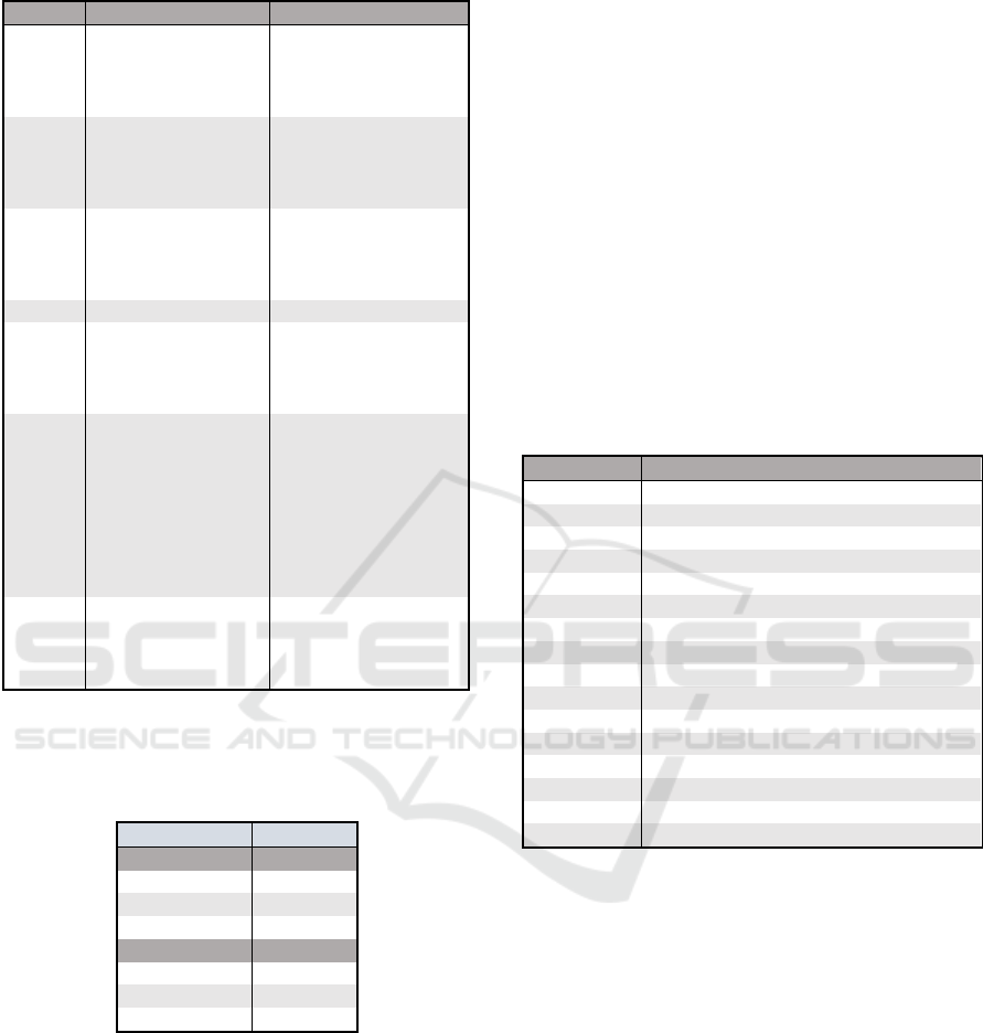
Table 3: Main experiment, adversarial attack parameters.

Attack Parameter Value

DNN init_epsilon 1 or 255 (depending

on ima

e bound

)

steps 200

amma 0.05

PGD rel_stepsize 0.025

abs

ste

size None

steps 50

random

start True

BIM rel_stepsize 0.2

abs

ste

size None

ste

s 10

random_start False

FGM random

start False

SLIDE quantile 0.99

rel

ste

size 0.2

abs_stepsize None

ste

s 50

BBA init_attac

None

overshoot 1.1

steps 100

0.001

lr_deca

0.5

num

deca

momentu

0.8

inar

ste

s 10

DF steps 100

candidates 10

overshoot 0.02

loss lo

its

Table 4: Epsilon values (perturbation sizes) used in the

experiment. The inception_v3 models requires the input

size to be 299x299x3 as opposed to 224x224x3 and has

been scaled appropriately.

pert. type value

not inception

l-inf 8

l-1 98,000

l-2 560

inception

l-inf 8

l-1 175,000

l-2 750

4 RESULTS AND DISCUSSION

16 attacks, 4 models and 1000 images were used to

generate 64,000 adversarial examples.

4.1 Attack Success Rates (ASR)

The attack success rates of each of the attacks was

obtained. From Table 5, it can be seen that adversarial

attacks are very effective on mobilenet, have similar

effectiveness against vgg16 and resnet50, and are less

effectiveness against inception_v3. This may be due

to the relative complexities of each of the neural

network architectures. Mobilenet’s lightweight

architecture appears to increase its vulnerability to

these adversarial attacks. On the other hand,

inception_v3’s more complex architecture appears to

increase its robustness against these attacks.

The FGM is a quick and basic attack involving

only a single step; as expected it has a lower ASR

compared to other attacks. The average ASR for each

model was:

Vgg16: 0.9679

Resnet50: 0.957625

Inception_v3: 0.8925

Mobilenet: 0.9907

Table 5: Attack Success Rates (ASR) of each adversarial

attack for each model (from 1000 images).

vgg16 rnet50 incep_v3 mnet

PGD_l1 0.968 0.991 0.946 0.999

PGD

l2 0.992 0.995 0.975 1.0

PGD

linf 1.0 0.999 0.999 0.999

BIM_l1 0.985 0.993 0.971 1.0

BIM

l2 0.998 0.994 0.988 1.0

BIM_linf 1.0 0.998 0.999 1.0

FGM

l1 0.875 0.837 0.588 0.959

FGM_l2 0.925 0.871 0.621 0.971

FGM

linf 0.977 0.924 0.663 0.983

SLIDE 1.0 0.998 1.0 1.0

DDN 0.948 0.93 0.999 0.998

DF_l2 0.909 0.876 0.805 0.969

linf 0.982 0.939 0.943 0.989

BBA_l1 0.946 0.989 0.793 0.991

BBA

l2 0.985 0.989 0.996 0.994

BBA_linf 0.996 0.999 0.994 0.999

4.2 Label Influence Analysis

Figure 1 shows an image of a pair of jeans and the

adversarial example generated from a PGD_l1

adversarial attack. The perturbation can be seen as

being quite sparse. It has only been scaled by 16

times. Small pockets in the perturbation image which

have a relatively high value can be seen, with the rest

of the image having no/minimal change. This is

expected from the l1 norm perturbation restriction

(sum of absolute values of all elements) and indicates

that these small pockets encourage the

misclassification the greatest.

For this image (and the other 999 images), 64

adversarial examples were created (4 models x 16

attacks). For the adversarial example shown in Figure

1, the adversarial label (top prediction of the resulting

adversarial example) was miniskirt. In fact, 63 of the

VISAPP 2021 - 16th International Conference on Computer Vision Theory and Applications

588

64 adversarial attacks for this image resulted in an

adversarial label of miniskirt. The remaining

adversarial label was hoopskirt.

Figure 1: Left: perturbation (x16) created using PGD_l1.

Top right: Clean, original image of a pair of jeans.

Bottom right: Adversarial example – misclassified as

miniskirt.

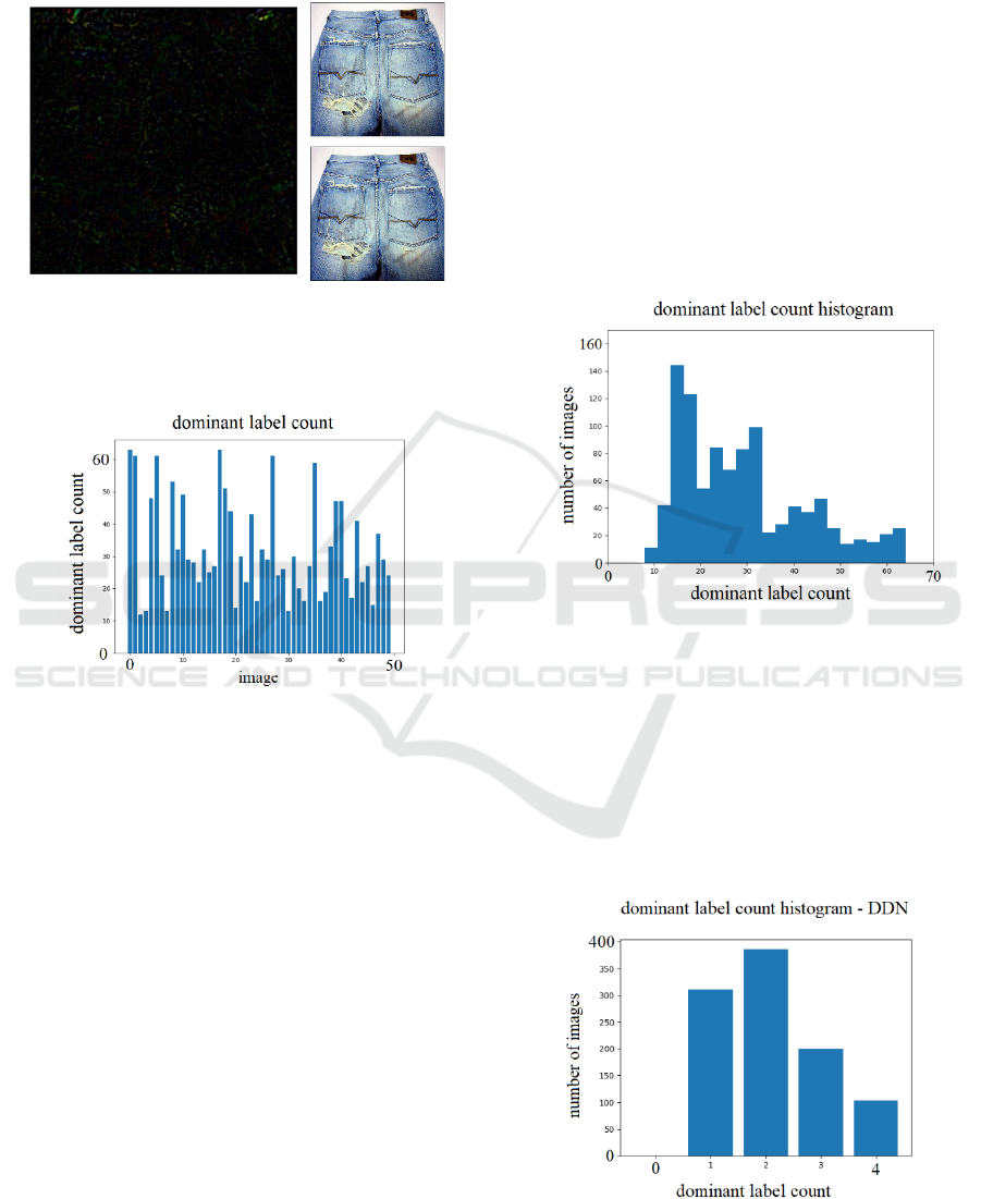
Figure 2: Plot of the number of times the most frequently

occurring label (dominant label) appears. For images 0 to

49.

From a set of adversarial examples (64 in this case)

of a single image, the ‘dominant label’ will be defined

as ‘the most frequently appearing adversarial label’.

The number of times the dominant label appears for

images 0 to 49 can be seen in Figure 2. For example,

the previous pair of jeans is image 0, the dominant

label is miniskirt and the number of times miniskirt

appears, or miniskirt count, is 63. This is represented

by the very first bar on the left.

From this plot, it can be seen that not all images

necessarily have a single dominant label. Images 2

and 3 have their dominant label only appearing 12 and

13 times. These images may have multiple

adversarial labels appearing as often, or almost as

often, as the dominant label.

The dominant label count of an image gives some

information about what influences the label. A high

count (e.g. image 0) means that regardless of the

attack and model, the resulting label is almost always

the same. In other words, the label is independent of

the attack and model, and only influenced by the

original image. On the other hand, a low count (e.g.

images 2 and 3), suggests that the adversarial label

isn’t greatly dependent on the original image.

The plot shown in Figure 2 can be extended for all

images from 0 to 999. A histogram of this extended

plot can be taken to visualize the dominant label count

of all 1000 images (Figure 3). The right-skewed

nature of the plot shows that most images have a low

dominant label count; the adversarial labels for these

images are not dependent just on the original image.

From this, it can be concluded that the image itself is

generally not a major influencer of the resulting

adversarial label.

Figure 3: Histogram of the number of images with each

dominant label count.

A similar histogram can be made with a focus on each

attack. Given a single adversarial attack, each image

now has 4 adversarial examples (from each model).

This can be seen in Figure 4 and Figure 5. The shape

of the histograms for all attacks are fairly similar. The

right skewed nature of all the plots once again

suggests that adversarial attacks do not have a large

influence over the resulting adversarial label.

Figure 4: Dominant label count histogram for the DDN

attack. 1000 images total, 4 attacks.

Analysing Adversarial Examples for Deep Learning

589

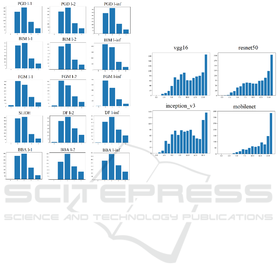
Figure 5: Dominant label count histograms for each

adversarial attack. Axes of each plot match Figure 4.

The same can be done with a focus on each model.

Given a single model, each image now has 16

adversarial examples (from each adversarial attack).

From Figure 6, it can be seen that these histograms

are left skewed. The images at the right end of the

histograms have a single adversarial label appear 15

or 16 times. For these images, regardless of the

adversarial attack, the resulting adversarial label is

the same.

From all these histograms it can be concluded that

the models, rather than the attacks, is the main

influencer of the resulting adversarial label, for a

given image. One potential explanation for this result

is that the attacks used were all gradient-based

attacks, which means the underlying algorithm for all

of these attacks are the similar; thus, all attacks cause

similar behaviors.

Comparing the models in Figure 6, mobilenet has

the ‘cleanest’ left skew, and inception_v3 appears to

be a normal distribution mixed with a left skewed

plot. The shapes of the other 2 models lie between

these 2 examples. The differences are likely due to the

differing network architectures. A light-weight

architecture seems to result in more consistent

adversarial label results.

By gaining insight into what influences the label,

i.e. the models, and the relationship between the

neural network architecture and the resulting

adversarial label, future defense techniques may be

able to use this information to better defend against

these untargeted attacks.

Figure 6: Dominant label count histograms for each model.

y-axis - number of images. x-axis - number of times most

freq. label appears (ranges from 0 to 16).

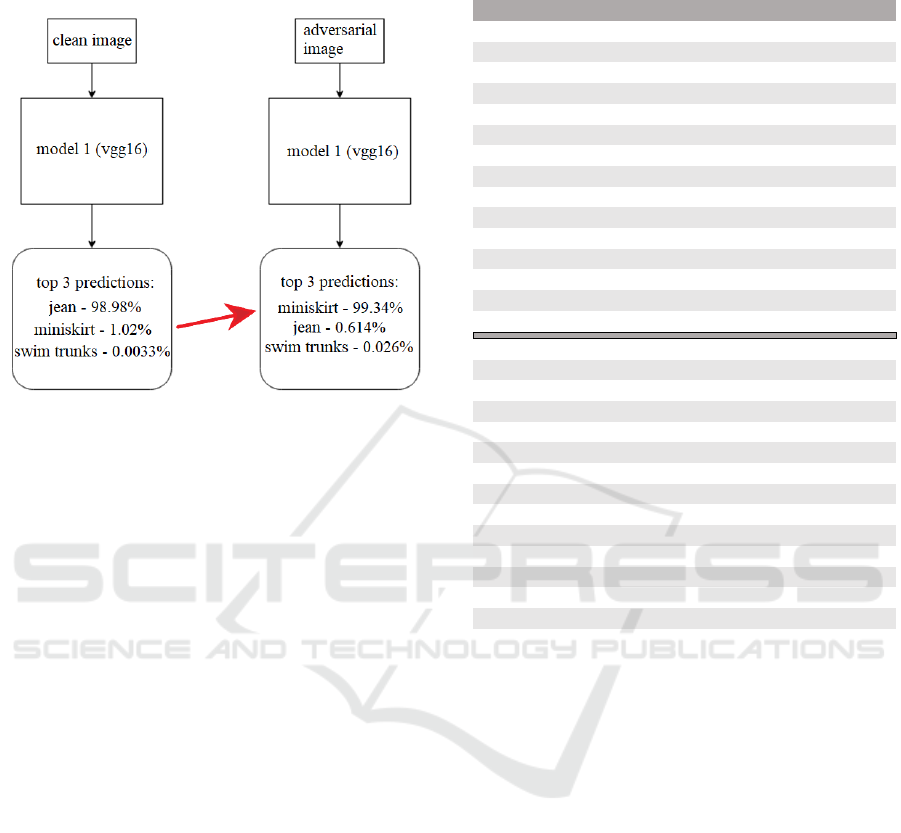
4.3 Label Movement Analysis

The movement of labels was also investigated. The

movement of labels refers to how the top label

predictions of the clean image may transfer to the top

predictions of the adversarial example. An example

diagram can be seen in Figure 7. The 2nd label or 2nd

highest prediction of the original image 0 is miniskirt

with a confidence of 1.02%, this becomes the

adversarial label or top prediction of the

corresponding adversarial image with a confidence of

99.34%.

Out of all 64,000 adversarial examples, it was

found that 52.2% of the 2nd label of the clean image

became the top prediction of the adversarial example.

12.2%, 5.8%, 3.4% of the 3rd, 4th and 5th labels of

the clean image become the top adversarial label.

4.7% of the time resulted in no label change (i.e.

adversarial attack failed), and 21.62% of the time

labels 6th – 1000th became the top prediction. Given

1000 possible classes, having the adversarial

examples’ top labels coming from the 2nd label of the

original images about half the time is a significant

result. Since the top predictions of the clean, original

image is only dependent on the image and model (and

not on the adversarial attack), the model and image

have a major influence on the resulting top

adversarial prediction/label.

VISAPP 2021 - 16th International Conference on Computer Vision Theory and Applications

590

This result supplements the previous result

showing that models influence the resulting label.

Figure 7: Label movement example for image 0. Top 3

predictions for the clean image (left) and adversarial

example (PGD_l1) (right).

4.4 Compare Attack Labels

The adversarial labels for each attack was compared

with each other attack, for each model. For each pair

of attacks, the number of adversarial labels which

match (out of 1000 images) was recorded. The top

and bottom 15 matches can be seen in Table 6.

The top pairs of attacks in Table 6 are very similar

attacks. The algorithms of the BIM, PGD and FGM

attacks are extensions of one another. It would be

expected that the resulting labels for these attacks

would often match. On the other hand, the bottom half

shows pairs of very different attacks, resulting in few

matching labels. Also, worth noting is that

inception_v3 appears often as the model with these

low matching pairs of attacks. It may be due to its

higher complexity which may encourage more

variety in the adversarial labels. Mobilenet appears

often at the top of Table 6 also suggesting once again

that the light-weight network results in the same

adversarial labels.

Table 6: Number of matching labels between pairs of

attacks. List of top 15 and bottom 15.

model attack 1 attack 2 No. matches

mobilenet BIM

l1 BIM

l2 973

resnet50 BIM_l1 BIM_l2 947

mobilenet PGD

l1 BIM

l1 933

mobilenet PGD_l1 PGD_l2 931

16 BIM

l1 BIM

l2 924

resnet50 FGM_l1 FGM_l2 919

mobilenet PGD

l1 BIM

l2 917

mobilenet BIM_l1 PGD_l2 916

mobilenet FGM

l1 FGM

l2 915

ince

tion

v3 FGM

l1 FGM

l2 913

resnet50 PGD_l1 PGD_l2 904

mobilenet PGD

l2 BIM

l2 903

mobilenet DDN BIM_l2 901

mobilenet BIM

l1 DDN 899

vgg16 PGD_l1 PGD_l2 890

ince

tion

v3 BIM

l1 BBA

l1 364

inception_v3 PGD_linf FGM_linf 363

ince

tion

v3 SLIDE FGM

linf 357

inception_v3 FGM_linf BBA_linf 355

ince

tion

v3 BBA

l1 BIM

l2 352

ince

tion

v3 BBA

l2 FGM

linf 348

inception_v3 DDN FGM_linf 345

16 BBA

l1 BIM

linf 343

vgg16 BBA_l2 FGM_linf 343

ince

tion

v3 SLIDE BBA

l1 343

vgg16 FGM_linf BBA_linf 336

ince

tion

v3 BBA

l1 PGD

linf 330

inception_v3 BBA_l1 FGM_linf 316

ince

tion

v3 BBA

l1 BIM

linf 280

vgg16 BBA_l1 FGM_linf 274

5 DISCUSSION

The results from the experiment have shown that the

neural network models have more influence over the

resulting adversarial label as opposed to the

adversarial attack. In addition, a simpler, more light-

weight network architecture can be seen as being

more susceptible to attacks and results in the same

labels for many different attacks. This may be

explained by considering the classification space of

the models.

The classification space is a high dimensional

space where each position in this space maps to a

label. An image in this space would be classified by

placing it into this space and checking the mapping.

By adding perturbations, the goal of adversarial

attacks is to adjust the position of the image just

enough to change the region (or label) in this

classification space. To explain the differences found

in this experiment, a light-weight network may have

relatively large regions of distinct labels in this

Analysing Adversarial Examples for Deep Learning

591

classification space which are spaced apart as

opposed to interwoven classification regions. This is

illustrated in Figure 8. For the light-weight network,

once the perturbation has caused the image to reach a

new classification region, it has a large margin of

error before accidently switching labels to another or

even back to the original label. However, the more

complex network requires much more finesse, as a

slight change may cause the image to move into

another classification region. Assuming the initial

epsilon specified was enough to reach a new

classification region, this would explain the high ASR

against the light-weight mobilenet model and the

lower ASR against the more complex inception_v3

model. This would also explain why using different

attacks against the light-weight model often resulted

in the same label; given the attacks are similar (all

gradient-based), even with slight differences there is

a high chance they all end up in the same large

classification region.

Figure 8: 2D illustration of classification space for a light-

weight (left) and complex (right) network. Each colour

represents a different label or classification region.

These insights found in this work may assist future

researchers to develop more robust models against

untargeted gradient-based attacks. Since the analyzed

attacks were all gradient-based, future work would be

to consider other attack types as well. Additional

research into the classification space of the models for

the ImageNet models should also be considered. For

example, comparing the classification space of

simpler and more complex neural network models.

ACKNOWLEDGEMENT

This work was supported in part by Defence

Advanced Research Projects Agency (DARPA)

under the grant UTrap: University Transferrable

Perturbations for Machine Vision Disruption. The

U.S. Government is authorized to reproduce and

distribute reprints for Government purposes

notwithstanding any copyright annotation thereon.

The views and conclusions contained herein are those

of the authors and should not be interpreted as

necessarily representing the official policies or

endorsements, either expressed or implied, of

DARPA, or the U.S. Government.

REFERENCES

Akhtar, N., & Mian, A. (2018, Mar 28). Threat of

Adversarial Attacks on Deep Learning in Computer

Vision: A Survey. Retrieved from

https://arxiv.org/abs/1801.00553

Brendel, W., Rauber, J., Kümmerer, M., Ustyuzhaninov, I.,

& Bethge, M. (2019, Dec 12). Accurate, reliable and

fast robustness evaluation. Retrieved from

https://arxiv.org/abs/1907.01003

Eykholt, K., Evtimov, I., Fernandes, E., Li, B., Rahmati, A.,

Xiao, C., . . . Song, D. (2018, Apr 10). Robust Physical-

World Attacks on Deep Learning Models. Retrieved

from https://arxiv.org/abs/1707.08945

Goodfellow, I. J., Shlens, J., & Szegedy, C. (2015, Mar 20).

Explaining and Harnessing Adversarial Examples.

Retrieved from https://arxiv.org/abs/1412.6572

Kurakin, A., Goodfellow, I. J., & Bengio, S. (2017, Feb 11).

Adversarial Examples in the Physical World. Retrieved

from https://arxiv.org/abs/1607.02533

Madry, A., Makelov, A., Schmidt, L., Tsipras, D., & Vladu,

A. (2019, Sep 4). Towards Deep Learning Models

Resistant to Adversarial. Retrieved from

https://arxiv.org/abs/1706.06083

Moosavi-Dezfooli, S.-M., Fawzi, A., & Frossard, P. (2016,

Jul 4). DeepFool: a simple and accurate method to fool

deep neural networks. Retrieved from

https://arxiv.org/abs/1511.04599

Rauber, J., Zimmermann, R., Bethge, M., & Brendel, W.

(2020). Foolbox Native: Fast adversarial attacks to

benchmark the robustness of machine learning models

in PyTorch, Tensorflow and JAX. Retrieved from

https://joss.theoj.org/papers/10.21105/joss.02607

Rony, J., Hafemann, L. G., Oliveira, L. S., Ayed, I. B.,

Sabourin, R., & Granger, E. (2019, Apr 3). Decoupling

Direction and Norm for Efficient Gradient-Based L2

Adversarial Attacks and Defenses. Retrieved from

https://arxiv.org/abs/1811.09600

Szegedy, C., Zaremba, W., Sutskever, I., Bruna, J., Erhan,

D., Goodfellow, I., & Fergus, R. (2014, Feb 19).

Intruiging properties of neural networks. Retrieved

from https://arxiv.org/abs/1312.6199

Tramèr, F., & Boneh, D. (2019, Oct 18). Adversarial

Training and Robustness for Multiple Perturbations.

Retrieved from https://arxiv.org/abs/1904.13000.

VISAPP 2021 - 16th International Conference on Computer Vision Theory and Applications

592