Distributed Service Area Control for Ride Sharing by using Multi-Agent

Deep Reinforcement Learning

Naoki Yoshida

, Itsuki Noda

2 a

and Toshiharu Sugawara

1 b

Computer Science and Engineering, Waseda University, Tokyo 1698555, Japan

National Institute of Advanced Industrial Science and Technology, Ibaraki 3058560, Japan

Keywords:

Multi-Agent Learning, Transportation and Logistics, Ride Sharing, Deep Reinforcement Learning.

Abstract:

We propose a decentralized system to determine where ride-sharing vehicle agents should wait for passengers

using multi-agent deep reinforcement learning. Although numerous drivers have begun participating in ride-

sharing services as the demand for these services has increased, much of their time is idle. The result is

not only inefﬁciency but also wasted energy and increased trafﬁc congestion in metropolitan area, while also

causing a shortage of ride-sharing vehicles in the surrounding areas. We therefore developed the distributed

service area adaptation method for ride sharing (dSAAMS) to decide the areas where each agent should

wait for passengers through deep reinforcement learning based on the networks of individual agents and the

demand prediction data provided by an external system. We evaluated the performance and characteristics

of our proposed method in a simulated environment with varied demand occurrence patterns and by using

actual data obtained in the Manhattan area. We compare the performance of our method to that of other

conventional methods and the centralized version of the dSAAMS. Our experiments indicate that by using the

dSAAMS, agents individually wait and move more effectively around their service territory, provide better

quality service, and exhibit better performance in dynamically changing environments than when using the

comparison methods.

1 INTRODUCTION

With advances in computer and communication tech-

nologies and the expanded use of smartphones with

the global positioning system (GPS), on-demand ride-

sharing services have become widespread and have

begun to attract many users. Because ride sharing al-

lows passengers who do not know one another to ride

in a single taxi/car, it increases their access to low-

priced transportation. Moreover, ride-sharing ser-

vices are expected to reduce both the number of cars

in a city area and the operational cost of services.

Ride sharing therefore provides advantages on both

the customer side and the provider side, and as a

result, ride sharing has been adopted by numerous

users (Yaraghi and Ravi, 2017) while the number of

participating companies, such as Uber and Lyft

, has

also increased.

Nevertheless, congestion is likely in urban and

https://orcid.org/0000-0003-1987-5336

https://orcid.org/0000-0002-9271-4507

https://www.uber.com/ and https://www.lyft.com/

busy areas due to the excessive number of taxis and

ride-sharing vehicles thanks to the rapid growth of

ride-sharing services (Erhardt et al., 2019). For exam-

ple, to increase their earnings, drivers tend to gather

around shopping areas, train stations, and airports,

where they can most easily ﬁnd passengers. This does

not cause a problem if the number of drivers is appro-

priate to the demands of the area. However, it is dif-

ﬁcult to maintain an appropriate number of drivers in

a given area and coordinate with each other to avoid

congestion. As a result, a supply bias may occur:

there may be both an oversupply of drivers in urban

areas, causing congestion, and a shortage of drivers

in suburban or residential areas, causing opportunity

loss.

In the recent years, there have been many studies

on taxi demand forecasting that analyze information

obtained from smart phones with GPS about where

people get in and out of taxis (Ke et al., 2017; Ma

et al., 2019). If a service provider can predict pas-

senger boarding and alighting points in advance using

forecasting information, the supply bias can be par-

tially solved by controlling the location of individual

Yoshida, N., Noda, I. and Sugawara, T.

Distributed Service Area Control for Ride Sharing by using Multi-Agent Deep Reinforcement Learning.

DOI: 10.5220/0010310901010112

In Proceedings of the 13th International Conference on Agents and Artiﬁcial Intelligence (ICAART 2021) - Volume 1, pages 101-112

ISBN: 978-989-758-484-8

101

cars. For example, Miao et al. (Miao et al., 2015) and

Iglesias et al. (Iglesias et al., 2017) proposed methods

to reduce the difference between the number of de-

mands and the number of taxis in an area by using de-

mand forecast information. However, taxi allocation

that strictly follows the demand forecast is vulnera-

ble because such the forecasting data usually contain

errors, actual demand is always ﬂuctuating, and taxi

demands may occur unexpectedly in inactive areas.

To improve the robustness of allocation methods

to data errors and dispersion, we have already pro-

posed the service area adaptation method for ride

sharing (SAAMS) as a control method for determin-

ing service areas, which are the areas where idle (so

empty) agents are to wait for future passengers, using

deep reinforcement learning (DRL) (Yoshida et al.,

2020), where agents driving control programs by as-

suming future self-driving vehicles. The neural net-

work in the SAAMS provides information about the

waiting areas for all independent agents based on the

demand forecast data. Although the SAAMS out-

performs conventional methods, it was designed as

a centralized system to be operated by a ride-sharing

company that would distribute the information to their

agents. When considering the actual usage and opera-

tion of ride-sharing services, it seems better for agents

to be able to independently choose their waiting area

to maximize their individual earnings, which are usu-

ally determined by the number of passengers to whom

they give rides. Furthermore, because a centralized

network requires the input information to be sent from

all agents and must then output the joint action of all

agents, its structure must be modiﬁed if the number of

agents changes, requiring a new learning process.

We therefore propose the distributed SAAMS

(dSAAMS) for each agent to improve the applica-

bility to actual operations and to improve the overall

proﬁts. Whereas the complexity of a centralized net-

work grows in accordance with the number of agents,

the independent network treats other agents as part of

the environment. Thus, the network structure does

not need to be changed when the number of agents

changes and that it is less complex. Nevertheless, it is

possible for the method to not converge due to its non-

stationarity and instability. Thus, in this paper, we ex-

perimentally show that it can converge and that coor-

dination and cooperation emerge even without giving

additional rewards to promote cooperation. We also

show that the dSAAMS can adapt to complex sim-

ulated environments in which demand is generated

in static and dynamic manners. Finally, we examine

its performance on a benchmark dataset obtained in

Manhattan, New York City (NYC).

2 RELATED WORK

Several different ride-sharing systems have been pro-

posed and studied. Before the 2010s, dial-a-ride on-

demand bus systems attracted attention, and many

methods were proposed to ﬁnd (near) optimal solu-

tions for arranging buses to minimize the travel and

waiting times (Cordeau and Laporte, 2003; Berbeglia

et al., 2012). Then, with the proliferation of mobile

devices, research has shifted to the problem of taxi

placement to anticipate passengers in ride-sharing ser-

vices (Nakashima et al., 2013; Alonso-Mora et al.,

2017). For example, Nakashima et al. (Nakashima

et al., 2013) proposed a ride-sharing service system

that seeks a reasonable arrangement of vehicles by (1)

sending a passenger’s demand to all cars, (2) calcu-

lating the expected trip time, including waiting time

and travel time, for each car, and (3) assigning the

demand to the vehicle with the shortest expected trip

time. They demonstrated that their allocation method

worked well experimentally for an actual ride-sharing

system in Hakodate City, Japan. Alonso-Mora et

al. (Alonso-Mora et al., 2017) proposed a method to

formulate taxi allocation in ride-sharing services in

the framework of integer programming in order to ob-

tain a semi-optimal solution. They showed that their

solution can reduce the number of taxis needed to

cover demand in NYC by 70%.

Meanwhile, there have been many studies on de-

mand forecasting for ride-sharing services (Ke et al.,

2017; Ma et al., 2019), and forecasting data have been

used in ride-sharing systems in recent years. Because

an imbalance between driver supply and passenger

demand leads to reduced efﬁciency and unnecessary

trafﬁc congestion, Miao et al. (Miao et al., 2015) pro-

posed the receding horizon control approach (RHC),

which is a position control method that uses the linear

programming framework to minimize the difference

between demand and supply using forecast data. They

have showed that their method can achieve efﬁciency

by dispatching empty taxis to expected busy areas.

However, by closely following the demand forecast,

this dispatch solution is not robust to errors contained

in the forecast.

Thanks to recent progress in research on DRL, es-

pecially deep Q-networks (DQNs) (Mnih et al., 2015),

It has been widely used to, for example, learn the

control of autonomous game playing and robot move-

ments even in complicated environments (Silver et al.,

2018; Akkaya et al., 2019). The use of the DQNs has

also been proposed in a number of studies on ride-

sharing systems (Lin et al., 2018; Oda and Joe-Wong,

2018; Wen et al., 2017), in which the proposed meth-

ods achieved similar or better allocation efﬁciency

ICAART 2021 - 13th International Conference on Agents and Artiﬁcial Intelligence

102

△△

△

Passenger

△

Car

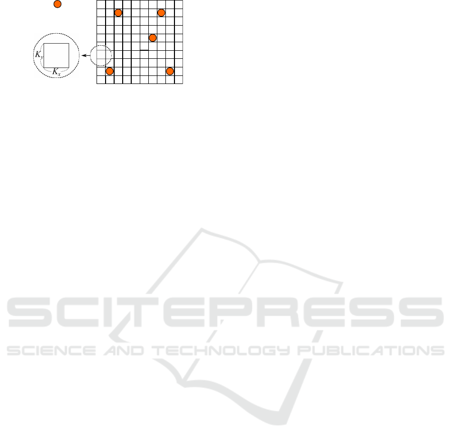
Figure 1: Environment of the ride-sharing problem.

than conventional methods that did not use the DQNs.

The systems proposed by Lin et al. (Lin et al., 2018)

and Oda et al. (Oda and Joe-Wong, 2018) have cen-

tralized deep networks, like the SAAMS (Yoshida

et al., 2020), that needed to learn micro-movements

in their environments (such as a sequence of mov-

ing up, down, left, and right) to generate the opti-

mal routes for traveling to destinations. As a result,

the learning was inefﬁcient because the appropriate

route selection was not easy to learn due to the dy-

namic and complicated road conditions. Wen, Zhao,

and Jaillet (Wen et al., 2017) proposed the rebalancing

shared mobility-on-demand (RSM) system in which

agents have their own DQNs by combining the de-

mand forecast data and dynamically control indepen-

dently when empty, to reduce the difference between

supply and demand. Moreover, the networks provide

the micro-movements to control themselves. How-

ever, these studies did not investigate the mechanism

behind the improvements in performance.

In contrast, the dSAAMS that we propose here

does not provide micro-movements and eliminates

route selection by assuming these activities are

learned in other components. Instead, it focuses on

the learning how to decide the service area of each

agent. This approach makes the learning efﬁcient and

enables the driver agents to follow the dynamics of

the environment.

3 PROBLEM AND MODEL

3.1 Problem Formulation and Issues in

SAAMS

We formulate the car dispatch problem for ride shar-

ing. We denote the set of agents by D = {1,...,n} and

introduce a discrete time t ≥ 0, for which one unit

of time, called a step, corresponds to approximately

2 to 3 min in our study. The environment is repre-

sented by an L × L grid (L ≥ 0 is an integer). Each

cell in the grid represents a K

×K

region (K

and K

are assumed to be approximately 500 m in the experi-

ments below). Fig. 1 shows an example environment,

in which the red circles represent agents and the tri-

angles represent passengers waiting for taxis. At each

time step, agent i can move up, down, left, or right by

one cell or can stay in their current cell. The goal of

this problem is for agents to pick up passengers from

their waiting places and deliver them to their desti-

nations in order to maximize their earnings. Agent

i ∈ D has a vehicle capacity Z

≥ 0 and cannot trans-

port more than Z

passengers. Let S be the set of states

of the environment. We denote the state at time t by

∈ S which includes all agents; the known passen-

gers in the environment; the current service areas of

all agents, which are be deﬁned below; and the most

updated demand prediction data, provided every 30

steps by a forecasting system outside the SAAMS.

Conceptual diagrams of the ride-sharing systems

with the SAAMS is shown in Fig. 2. At time t, the

ride-sharing company operates the SAAMS to con-

trol all agents that belong to it. The SAAMS has the

centralized DQN whose input consists of states of all

agents, their received rewards and the forecast data.

It then assigns agent i (for ∀i ∈ D) to its service area

i,t+1

for next time, which are a subset of the envi-

ronment. When a passenger requests a taxi in a given

location, the operator in the company assigns the most

appropriate (i.e., the closest) agent whose service area

includes the passenger’s current location.

Agent i then attempts to move to the service area

(preferably, to its center) if its vehicle is empty. When

the vehicle of agent i is not empty (i.e., they are trans-

porting passengers or have been assigned passengers),

they continue their current service (i.e., they continue

driving to the passengers’ destination or waiting area).

After dropping off all passengers, agent i returns to

the center of C

i,t

. That is, the SAAMS indirectly nav-

igates the agents by ﬂexibly changing the service area

locations. The SAAMS adjusts the position and size

of C

i,t

to improve the quality of the service and to in-

crease the total beneﬁts. Meanwhile, the agents do

not independently change their service area and in-

stead wait for updates from the SAAMS.

3.2 Dispatch Management using

Distributed SAAMS

The SAAMS is a centralized controller for a ride-

sharing company. It may be able to coordinate be-

havior to some degree, i.e., a few agents may be al-

located to unbusy areas to provide better service for

rare demands even though these agents are likely to

remain idle. However, if the agents’ income is based

on commission in the ride-sharing service, it is more

appropriate for agents to autonomously choose their

service areas, even if they belong to the same com-

Distributed Service Area Control for Ride Sharing by using Multi-Agent Deep Reinforcement Learning

103

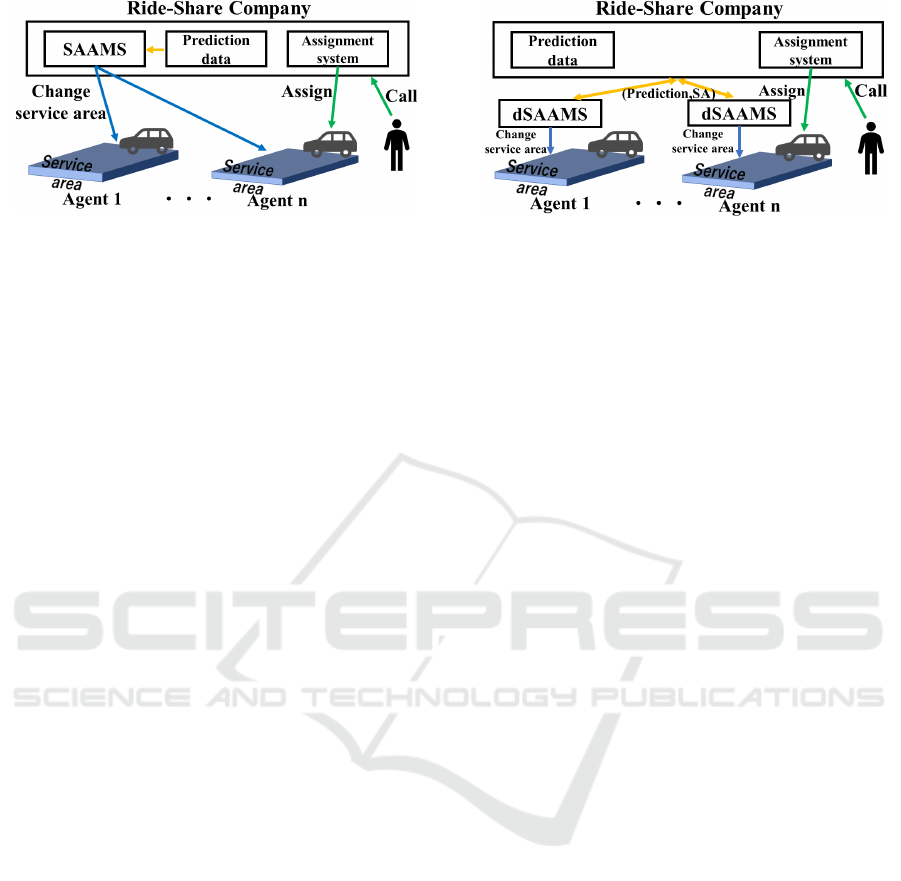
Figure 2: The SAAMS taxi dispatch system.

pany. Another drawback of SAAMS is that the struc-

ture of input has to change in accordance with the

increase of agents; this often occurs in a real-world

ride-sharing service company where more than a few

hundred agents are involved and the number of agents

is likely to change. Therefore, the network must be

reconﬁgured and need to be trained again. For this

reason, the central control of the SAAMS seems un-

suitable for real-world operations.

We thus introduced the dSAAMS, as shown in

Fig. 3. Agents in the dSAAMS may work for the

same company but they individually learn using their

own network to appropriately select their service ar-

eas by themselves. This system architecture makes

this method more ﬂexible and widely applicable be-

cause the network structure is not affected by the

number of agents that belong to a company. How

to assign a request from passengers to the appropri-

ate agents is identical to that by the company us-

ing the SAAMS. The main concerns are whether the

dSAAMS can learn excellent (or at least acceptable)

strategies for determining service areas and the con-

vergence and stability of these strategies. A perfor-

mance comparison between the dSAAMS and a con-

ventional method (Wen et al., 2017) is also of inter-

est because the distributed setting of the conventional

method is quite similar to the method used in our

method.

When a ride-sharing company receives a request

from a group of passengers at time t, it immediately

attempts to assign the request to an agent i ∈ D who

meets the following conditions:

(a) Agent i is a vacant agent; that is, its vehicle is

empty or has enough empty seats for the new pas-

sengers (the capacity limit Z

cannot be violated);

(b) The service area C

i,t

of i includes the place where

the passengers are waiting; and

where the passengers are waiting.

Because it may take extra time to pick up passengers

for carpooling, it is assumed that the time required

for carpooling passengers to board is twice as long as

Figure 3: The dSAAMS taxi dispatch system.

for a non-carpooling ride. This assignment process

requires that the ride-sharing company receive infor-

mation about the service areas of all agents, whereas

a ride-sharing company using the SAAMS determines

the service areas in a centralized way and distributes

them.

To avoid extreme detours that could be caused by

ride sharing with other passengers, we introduce the

additional condition of the expected maximum travel

time (EMTT). The EMTT is speciﬁed by the upper-

limit factor T

(≥ 1). The EMTT condition is

The expected travel time for carpooling must not

exceed T

times the expected travel time for a

non-carpooling ride.

is set by the ride-sharing company to maintain

its service quality. The company only assigns agents

such that the EMTT condition is not violated. If more

than one agent meets the conditions, the dispatch sys-

tem randomly selects one of them. When there is no

assignable agent, the passengers are immediately de-

clined, and service is not provided. When multiple

demands arrive, they are processed sequentially by

the ride-sharing company. When agent i is assigned

passengers, they move to the waiting area, pick up the

passengers, drive to the destination, and drop off the

passengers. After that, agent i returns to their service

area.

In this study, the agents try to maximize the earn-

ings of the ride-sharing company, which is the sum

of the proﬁts of the individual agents. On their own,

the agents would likely congregate in areas with high

demand to increase their personal earnings. How-

ever, this concentration can result in excessive com-

petition and many agents remaining idle. Moreover,

it also causes a lack of service in those areas where

demands occur infrequently. To avoid this, in our

system, agents learn coordinated behavior using their

own networks.

ICAART 2021 - 13th International Conference on Agents and Artiﬁcial Intelligence

104

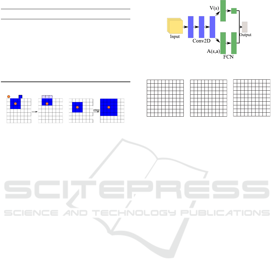
Table 1: List of adjustments to a service area.

Name Manipulation to adjust C

Enlarge C

, of size T

× T

, is enlarged to size

+ 2) × (T

+ 2).

Shrink C

, of size T

× T

, is shrunk to size

− 2) × (T

− 2).

Up, down,

left, right

is moved up, down, left, or right

(without a change in size).

Stay The size and location of C

are main-

tained.

Car

Service Area

(a) up adjustment of C

(b) enlarge adjustment of C

Figure 4: Examples of manipulations for service areas.

3.3 Service Area and Its Adjustment

Agents using the dSAAMS adjust their service area

to increase earnings as well as to provide quality ser-

vice. Let A be the set of the manipulations to adjust

service area C

i,t

for agent i ∈ D. The service area C

i,t

is a rectangular area of cells (a square in the experi-

ments below) with a maximum size of T

× T

, where

L ≥ T

≥ 1 are integers, and the minimum area

is 1 × 1. An adjustment a

∈ A at time t is one of

A = {enlarge,shrink,up,down,left,right,stay}; the

details of these adjustments are listed in Table 1. Ex-

amples of the adjustments up and enlarge are shown

in Fig. 4. Note that since agents are directed to move

to the center of their service area, after an up manip-

ulation of the service area as in Fig. 4a, the agent will

try to move up in next step if possible. If an adjust-

ment of C

i,t

would result in a violation of the size con-

straints, the selected adjustment is stay. Agents’ cur-

rent locations and the manipulations on their service

areas may be independent because if they are on their

way to drop off passengers, they may be far from their

service areas.

4 PROPOSED METHOD

4.1 Learning in dSAAMS

The DQN of the dSAAMS of agent i learns manipula-

tions to adjust C

i,t

to maximize the estimated rewards.

In this study, to balance the earnings and service qual-

Figure 5: Structure of the Dueling Neural Network in

dSAAMS.

(a) Prediction

data

(b) Individual ser-

vice area

1 1

3 3

3 3 3

4 4 4

5 5 5

vice area

Figure 6: Input to DQN.

ity, we introduce weighted rewards to agent i:

∑

p∈P

+ w

(1)

= −w

, (2)

where w

, w

, and w

are non-negative weights,

and P

is the set of passengers assigned to agent i at

time t. Parameter f

≥ 0 is the dispatch fee for passen-

ger p ∈ P

, parameter f

≥ 0 is the expected travel dis-

tance, and parameter f

≥ 0 is the service travel time

for passenger p. Since we assume that the routes are

determined using another mechanism, the travel dis-

tance and time are based on the shortest route between

two locations, and carpooling detours are not consid-

ered. Parameter f

≥ 0 is the cost of an empty agent

moving to a neighboring cell. We assume that r

(≥ 0)

is the reward (fare) obtained from passenger p. Agent

i receives r

only when they are assigned p, whereas

a negative reward (fuel expense) r

arises whenever

agent i moves to a neighboring cell. All agents inde-

pendently learn how to adjust their own service areas

to increase the total rewards of

∑

+ r

. Note that

since r

is negative, agents attempt to transport pas-

sengers for as long as possible. All parameters used

in Formulae (1) and (2) should be deﬁned by the ride-

sharing company.

4.2 Structure of Deep Q-Network

Because the proposed dSAAMS is a decentralized

control, where each agent learns behaviors indepen-

dently on the basis of locally earned rewards and ex-

pense, we have to verify if the decentralized control

by the dSAAMS converge.

Distributed Service Area Control for Ride Sharing by using Multi-Agent Deep Reinforcement Learning

105

The proposed DQN for the dSAAMS of each

agent is a dueling network (Wang et al., 2016), as

shown in Fig. 5, whose output is the combination of

the estimated values V(s) of state ∀s ∈ A and the ad-

vantages A(s, a) of a ∈ A in s. This network con-

sists of three convolutional layers (no pooling layers)

whose inputs to the ﬁrst layer are matrices represent-

ing the environment in an abstract way, and four fully

connected network (FCN) layers for the estimated

values and the advantages. The activation function is

the rectiﬁed linear unit (ReLU). When the service area

of agent i is modiﬁed, agent i sends that information

to the ride-sharing company for proper assignment.

Three types of L × L matrices form the input to

the network of agent ∀i ∈ D (example matrices are

shown in Fig. 6, where a blank cell in the matrices

except that of prediction data indicates zero). The

ﬁrst matrix includes the recent demand forecast data

from the demand forecast component. Its elements

are the demand forecast rates, which are non-negative

real numbers that indicate the expected number of de-

mands across 30 time steps at each cell. The blank

cells in Fig. 6a indicate uniform, low demand rates

(such as 0.1 and 0.025). The second matrix (Fig. 6b)

expresses the service area of agent i itself. The third

matrix (Fig. 6c) indicates the number of agents (in-

cluding that of agent i) whose service areas include

the corresponding cells. For example, a 5 indicates

that ﬁve agents include that cell in their service areas.

To generate the third matrix, we assume that the ride-

sharing company shares and distributes the service ar-

eas of all agents. This information is also needed for

the company to properly assign passenger demands to

appropriate agents.

5 EXPERIMENTAL EVALUATION

5.1 Experimental Setting

We experimentally evaluated the proposed method,

dSAAMS, in a simulation environment by compar-

ing it with other methods. Our experiments were

conducted in a 10 × 10 grid environment (L = 10,

see Fig. 7) using simulated scenarios and well-known

benchmark data obtained in Manhattan, NYC (NYC,

2020). We used a grid environment since it is sim-

ple and easy to understand to compare the features

of the methods used in our experiments. In addition,

the evaluation using the public benchmark dataset of

taxi trips in the Manhattan area allows us to evaluate

the performance of the methods in a real application.

The parameters of agent dSAAMS networks are listed

in Table 2. There were 2000 episodes in the train-

ing phase, and we used the ε-greedy learning strategy,

with a gradually decaying value of ε. The value of ε

in the N-th episode was 1.0 − 0.9N/2000, so ε was

gradually decreased to 0.1. ε = 0 in the testing phase.

We adopted the RHC (Miao et al., 2015), the

method used by Wen et al. in their RSM sys-

tem (referred to as the RSM hereafter) (Wen et al.,

2017), and SAAMS, which is the centralized version

of dSAAMS (Yoshida et al., 2020), as comparative

methods. The RHC tries to move unassigned cars

to areas with shortages by giving instructions based

on prediction data. It uses the linear programming

framework and has been often used for comparative

evaluation. We omitted the comparison with other

methods (Lin et al., 2018; Oda and Joe-Wong, 2018),

because they include the route selection, making a di-

rect performance comparison difﬁcult.

The RSM learns to control agents with their own

DQNs. Each DQN takes as input the demand fore-

cast matrices, the positions of nearby agents, and the

estimated total supply of cars. It then outputs the Q-

value for each movement. One difference between the

RSM and the dSAAMS is that the dSAAMS takes the

entire environment as its input (because it is a natu-

ral assumption that agents have maps of the service

territory). In contrast, the agents in the RSM only

get information about the local 5 × 5 grid centered

on their location (probably assuming local commu-

nication). The rewards in the RSM might increase if

the agents could quickly move to areas where passen-

gers are waiting after dropping off their current pas-

sengers.

We adopted three evaluation measures in the test-

ing phase: the operating proﬁts (OP), which are the

rewards from the passengers,

∑

t=1

∑

i∈D

, where L

is the episode length; the ratio of the waiting time

(RWT), i.e., the ratio of the required time in steps

to pick passengers up to the total travel time to their

destination; and the average travel distance per agent

(ATD) per episode, where the distance is deﬁned as

the number of cells, making this value identical to

= w

by setting f

= 1. The OP seems to be the

most important indicator for the ride-sharing com-

pany because it reﬂects the income of the company.

The reward weights for calculating r

and r

in the

dSAAMS training phase were set to w

= 3, w

= 0.2,

= 0.2, and w

= 0.05 by referring to actual ride-

sharing operations. The value of RWT represents the

ratio of the waiting time which is one aspect of service

quality, so a smaller value is better. A smaller value

of ATD is also better because it represents the average

fuel consumption per episode of individual agents.

ICAART 2021 - 13th International Conference on Agents and Artiﬁcial Intelligence

106

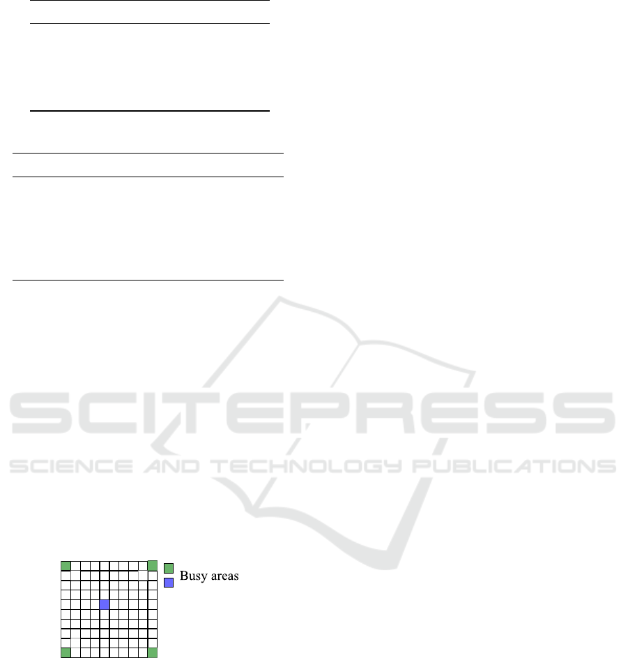
Table 2: Network parameters.

Parameter Value

Replay buffer size, d 20,000

Learning rate, α 0.0001

Update interval of target network 20,000

Discount factor, γ

0.99

Mini batch size, U 64

Table 3: Setup parameters.

Parameter Value

Number of agents, |D| = n 20

Episode length, L

150

Vehicle capacity, Z = Z

for ∀i ∈ D 4

Max. size of service area, T

Cost of moving to a neighboring cell, f

Upper-limit factor for EMTT, T

5.2 Simulated Grid Environments

We conducted the ﬁrst experiment (Exp. 1) in the sim-

ulated environment shown in Fig. 7, in which blue and

green cells correspond to busy areas/places such as

stations, halls, museums, shopping malls, and hospi-

tals. We prepared four scenarios with different pat-

terns in the demand occurrence rate in the grid envi-

ronment. The demand occurrence rate λ (> 0) in a cell

is deﬁned as the demands from passengers, which are

generated according to the Poisson distribution P

(λ)

every 30 steps (i.e., P

(λ/30) per step). Note that the

expected value of P

(λ) is λ. The passenger destina-

tions are assigned randomly unless stated otherwise.

Figure 7: Experimental environment.

In Scenario 1, the pattern is static: the demand oc-

currence rate is 4 (λ = 4) in each green cell and

is λ = 0.025 for the other cells. Therefore, 18.4

(0.025 × 96 + 4 × 4) demands are generated on av-

erage every 30 steps in the whole environment. Sce-

nario 2 is uniform: λ = 0.25 for all cells. In Scenario

3, the pattern is dynamic and biased: the blue cell

is a train station, and the four green cells correspond

to other busy places. There are many demands for

rides between the station and one of the busy cells.

Therefore, the blue cell or one of the green cells is

randomly selected every 30 steps, and its demand oc-

currence rate is set to λ = 12, while for the other cells

λ = 0.025. Any demand occurring at the blue cell has

its destination as one of green cells with a probability

of 0.98 (otherwise, the destination is random with a

probability of 0.02). Similarly, a demand occurring at

one of the green cells has the station (blue cell) as its

destination with a probability of 0.98, with the des-

tination being randomly selected otherwise. Finally,

the pattern in Scenario 4 is more dynamic, and its de-

mand occurrence rate varies every 30 steps as listed

in Table 4.

We assume that the demand forecast matrix is cor-

rect in the sense that its elements are identical to their

demand occurrence rate λ for the corresponding cells.

However, since the demands are generated randomly

according to P

(λ), the number of demands gener-

ated in a cell may not be equal to λ. Moreover, since

the updated demand forecast data are given every 30

steps, the same demand forecast matrix is provided to

the individual agent networks until the next update ar-

rives, whereas it may almost be obsoleted in the last

part of the interval. The other setup parameters for

Exp. 1 are listed in Table 3.

5.3 Performance Comparison

The results of all scenarios of Exp. 1 are listed in

Table 5. Table 5a indicates that agents using the

dSAAMS earned the highest OP. We can thus say

that the dSAAMS outperformed the other methods in

all scenarios. Another observation is that the decen-

tralized control systems, i.e., the dSAAMS and RSM

earned more OP than the centralized control systems.

The difference between the OP obtained using the

dSAAMS and that using the RSM was the largest

in Scenario 3. Because most of the passenger ﬂow

was unidirectional in this scenario, the movement of

agents using the dSAAMS, which returns agents to

their service areas after passengers are dropped off,

matched the ﬂow well. The difference between the

dSAAMS and RSM was second largest in Scenario 4.

In this scenario, the ﬂow of passengers was also dy-

namic, and its direction of movement was also some-

what biased. We believe that actual ﬂow is likely to be

biased, as in Scenarios 3 and 4, making the dSAAMS

better for real ride-sharing applications.

The ratio of the waiting time (RWT) and the av-

erage travel distance (ATD) are listed in Tables 5b

and 5c. The RSM produced the shortest values for

the RWT, with the SAAMS and dSAAMS produc-

ing relatively longer values. Because the environ-

ment of Scenario 2 is uniform and has no busy areas

Distributed Service Area Control for Ride Sharing by using Multi-Agent Deep Reinforcement Learning

107

Table 4: Demand occurrence rates in Scenario 4 (per 30 steps).

Cell (t =)0 to 29 30 to 59 60 to 89 90 to 119 120 to 149

Green 4 2.5 0.025 2.5 4

Blue 0.025 8 18 8 0.025

Others 0.025 0.025 0.025 0.025 0.025

Table 5: Performance Comparison.

(a) Received operating proﬁt (OP).

Scenario 1 Scenario 2 Scenario 3 Scenario 4

dSAAMS 682.7 801.3 510.3 728.7

SAAMS 594.0 690.3 406.5 591.4

RSM 660.4 771.9 440.9 680.6

RHC 631.9 766.1 464.9 619.4

(b) Ratio of the waiting time (RWT, %).

Scenario 1 Scenario 2 Scenario 3 Scenario 4

dSAAMS 5.3 18.9 13.0 9.3

SAAMS 10.1 10.5 13.3 10.2

RSM 4.6 10.5 11.2 5.2

RHC 11.0 17.1 11.3 11.0

Scenario 1 Scenario 2 Scenario 3 Scenario 4

dSAAMS 76.0 90.9 55.4 80.4

SAAMS 78.7 97.9 63.7 69.7

RSM 116.8 138.5 118.1 114.5

RHC 116.3 143.2 104.5 115.7

and because the (d)SAAMS includes the concept of

service areas, agents are occasionally far from their

service areas when dropping off passengers, meaning

that the passengers may have to wait longer. Never-

theless, the dSAAMS still earned the highest OP even

in Scenario 2 (Table 5a) and a uniform environment

is unrealistic. Table 5c shows that the agents using

the dSAAMS have the smallest ATD because agents

using the dSAAMS were likely to wait in their ser-

vice area, thereby avoiding unnecessary moves. The

dSAAMS is thus the most cost- and energy-effective

control system.

5.4 The Waiting Place Strategy

To investigate the waiting points of the agents, we

generated heatmaps that indicate the numbers of vis-

its to each cell in the grid by each agent in Sce-

nario 1 (since it is the simplest scenario, facilitat-

ing the understanding of the agent behavior). The

heatmaps for four agents are shown in Fig.8. We

selected four agents that they were likely to pick

up passengers from different busy cells. Since the

demand occurrence rates were high on four corner

cells, these agents, especially the agents using the

dSAAMS, were likely to visit and stay at one cor-

ner (Fig. 8a). The agents using the SAAMS exhib-

ited a similar tendency but wandered a little; their ser-

vice areas were probably strongly affected by the po-

sitions of other agents (Fig. 8b). The agents using the

RSM seemed to identify the busy corners (Fig. 8c),

but since they were not using the concept of service

areas, they were likely to wait for new passengers

at the destination of their previous passengers or in

crowded cells near those destinations. This type of

movement can be successful when all areas are busy,

in which case agents will soon be able to ﬁnd new

passengers. However, in some cases, agents using the

RSM had to wait in quiet areas or even in busy places;

that is, their waiting places could be biased. Under

ICAART 2021 - 13th International Conference on Agents and Artiﬁcial Intelligence

108

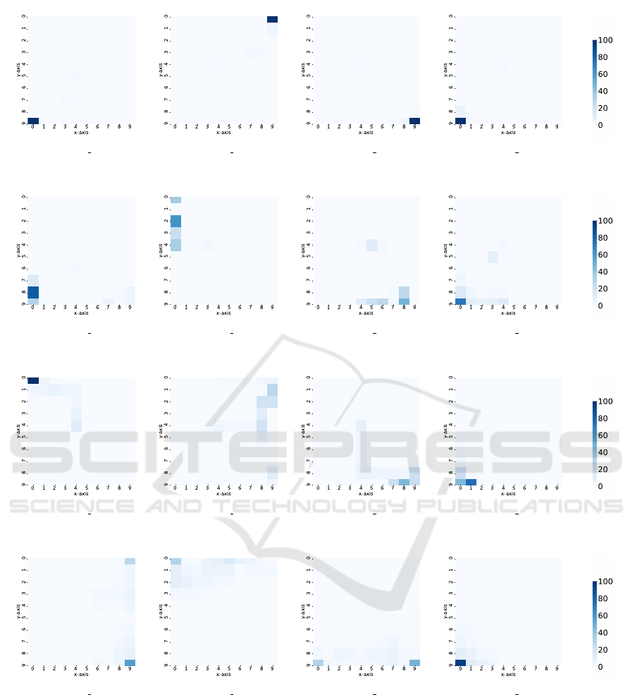
Agent 0 Agent 1 Agent 2 Agent 3

(a) dSAAMS

Agent 0 Agent 1 Agent 2 Agent 3

(b) SAAMS

Agent 0 Agent 1 Agent 2 Agent 3

(d) RHC.

Figure 8: Heatmap of agent locations in an episode of the testing phase.

the control of the RHC approach, the waiting loca-

tions changed more frequently (Fig. 8d) because for

example, when agents with passengers moved to their

destinations, other empty agents near the destination

would move away to maintain the strict balance be-

tween the number of agents in busy cells.

To investigate the strategies of the agents with the

dSAAMS more thoroughly, we generated a snapshot

of the service areas of all the agents at a certain time

step. A snapshot of the 30th time step is shown in

Fig. 9. We can see that the agents attempted to set

their service areas to cover the whole environment.

The service areas of almost all agents include one of

the busy cells, while two agents (5 and 9) covered less

busy cells with relatively wider service areas (the size

of the service areas was limited by T

and T

, which

Distributed Service Area Control for Ride Sharing by using Multi-Agent Deep Reinforcement Learning

109

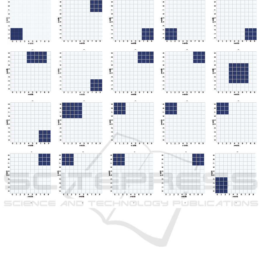
Agent 0

Agent 1 Agent 2 Agent 3 Agent 4

Agent 5

Agent 6

Agent 7 Agent 8 Agent 9

Agent 10 Agent 11 Agent 12 Agent 13 Agent 14

Agent 15 Agent 16 Agent 17 Agent 18 Agent 19

Figure 9: Snapshot of agent service areas with the dSAAMS.

were set to 5). Note that the location and size of the

service areas varied over time, and the agents were

thus able to accept almost all passenger demands.

5.5 Using Manhattan data

We also evaluated dSAAMS using real-world data

from Manhattan, with the RSM and RHC tested for

comparison in Exp. 2. The Manhattan area was di-

vided into regions of size 22×11, and it was assumed

to be a grid environment for our experiment. We used

data obtained from Feb. 1 to 14, 2018 for training and

data from Feb. 15 to 21, 2018 for testing. We set

the number of agents |D| to 100 due to the limited

computational resources. This is much smaller than

the number of yellow cabs in NYC, which is usu-

ally limited to around thirteen or fourteen thousand

(excluding ride-sharing vehicles, such as Uber and

Lyft). Although we could not determine the appro-

priate number of taxis and although some taxis might

not be operating at a given time, we randomly reduced

the data by selecting data points with a probability of

|D|/8000 = 0.0125 (8,000 is about 60% of 13,000, by

assuming about 60% of all taxis are in operation). We

assumed that one time step was one minute and that

the length of one episode was 1440 steps (L

= 1440),

which corresponds to one day. The update interval of

target network was thus also set to 1440. The num-

ber of episodes in the training phase was 100. Since

the training data cover only two weeks, the same data

were used multiple times. This training length may

seem short, but the learning almost converged. The

value of ε was decreased linearly from 1.0 to 0.1. The

other experimental parameters were identical to those

in Tables 2 and 3.

For Exp. 2, the demand forecast data were, as in

other studies (Oda and Joe-Wong, 2018), generated

by a neural network whose inputs are two matrices

that represent the distribution of passengers during the

previous two steps. The output is the demand forecast

data for next step. The ﬁrst layer consisted of thirty-

two 3 ×3 ﬁlters with a leaky rectiﬁed linear activation

ICAART 2021 - 13th International Conference on Agents and Artiﬁcial Intelligence

110

Table 6: Results for the Manhattan data.

Parameter OP RWT ATD

dSAAMS 16347.1 6.9 557.1

RSM 16072.8 10.6 1100.2

RHC 16055.3 15.7 1227.7

unit (leaky ReLU). The next layer consisted of sixty-

four 2 × 2 ﬁlters with a leaky ReLU. The last layer

was a 1 × 1 ﬁlter with the same activation function.

The forecast data were updated every 30 steps to es-

timate the demand occurrence rates for the next 30

steps.

The results are summarized in Table 6. This table

indicates that the dSAAMS exhibited the best perfor-

mance in these experiments. There are several rea-

sons for its relatively good performance. First, the

agents using the dSAAMS were able to accept and

meet almost all the passenger demands, whereas the

other methods were occasionally unable to accept a

few demands. This enabled agents using dSAAMS

to earn greater OP. Second, the RWT and ATD of the

dSAAMS were much smaller than for the other meth-

ods. The agents using the RSM were again likely to

wait for new passengers near the destination of their

previous passengers, but these places were not neces-

sarily busy. As a result, passengers were more likely

to have to wait longer.

The strategy learned with the RSM seems be ef-

fective when all areas are busy because agents can

pick up their next passengers where they drop off their

previous passengers. The full results are not provided

here, but if we change the probability of reduction of

data from 0.0125 to 0.05 (making the area four times

busier), the agents using the RSM generate slightly

more OP than the agents using the dSAAMS. This oc-

curs even though in an incredibly busy environment in

which many demands were rejected even when using

the RSM. We believe that such situations are not real-

istic and that the number of passengers per agent will

instead be relatively small due to the entry of other

ride-sharing companies into the business, increasing

the competition rate between agents in a ride-sharing

market of constant size.

5.6 Remark

Comparing the centralized and decentralized

SAAMSs, it seems that the dSAAMS can dispatch

agents more appropriately in static situations (such

as Scenarios 1 and 2) and can adapt more ﬂexibly to

changes in the environment (Scenarios 3 and 4) than

the SAAMS. The RSM, which is also decentralized,

also exhibited better performance than the SAAMS.

Although there were concerns about instability and

non-convergence due to the decisions being fully

decentralized, the networks converged for good

results. Fig. 8 shows that the dSAAMS prompted

fewer unnecessary movements than the SAAMS and

that it earned higher OP. Since the number of taxis in

operation always varies, we believe that the dSAAMS

can be efﬁcient for actual ride-sharing control.

6 CONCLUSION

To improve the applicability to actual operations and

the overall beneﬁts and efﬁciency of ride-sharing con-

trol, we propose the dSAAMS, in which each agent

uses their own deep Q-network to determine the ser-

vice area where they should wait for passengers. The

dSAAMS is a decentralized and extended version of

the SAAMS (Yoshida et al., 2020). Using dSAAMS,

we can easily increase the number of agents in a ride-

sharing company. In contrast, the centralized network

of the SAAMS controls all agents, and the structure

of the network must therefore be modiﬁed and re-

trained when a new agent is added. We conducted

experiments in simple simulated environments and in

a more complicated environment based on real data

acquired in Manhattan, New York. By learning the

service areas, the dSAAMS was able to reduce supply

shortages and biases, resulting in higher rewards and

reduced travel distances compared to existing meth-

ods.

One drawback of the dSAAMS is that it requires

a relatively long training time to obtain stable learn-

ing results when the number of agents is large, but we

believe that these calculations can be performed on a

large number of PCs in the cloud. We may also need

to use incremental learning, in which the number of

agents is gradually increased by adding new agents

that have no prior learned knowledge. Another pos-

sible approach is transfer learning, in which a small

number of agents learn in advance, and the number of

agents is then increased by transferring their knowl-

edge to new agents. These are the topics of our future

work.

ACKNOWLEDGEMENTS

This work was partly supported by JSPS KAKENHI

(17KT0044) and JST-Mirai Program Grant Number

JPMJMI19B5, Japan.

Distributed Service Area Control for Ride Sharing by using Multi-Agent Deep Reinforcement Learning

111

REFERENCES

Akkaya, I., Andrychowicz, M., Chociej, M., Litwin, M.,

McGrew, B., Petron, A., Paino, A., Plappert, M., Pow-

ell, G., Ribas, R., et al. (2019). Solving rubik’s cube

with a robot hand. arXiv preprint arXiv:1910.07113.

Alonso-Mora, J., Samaranayake, S., Wallar, A., Fraz-

zoli, E., and Rus, D. (2017). On-demand high-

capacity ride-sharing via dynamic trip-vehicle assign-

ment. Proc. of the National Academy of Sciences,

114(3):462–467.

Berbeglia, G., Cordeau, J.-F., and Laporte, G. (2012). A

hybrid tabu search and constraint programming algo-

rithm for the dynamic dial-a-ride problem. INFORMS

Journal on Computing, 24:343–355.

Cordeau, J.-F. and Laporte, G. (2003). A tabu search

heuristic for the static multi-vehicle dial-a-ride prob-

lem. Transportation Research Part B: Methodologi-

cal, 37(6):579 – 594.

Erhardt, G. D., Roy, S., Cooper, D., Sana, B., Chen, M.,

and Castiglione, J. (2019). Do transportation network

companies decrease or increase congestion? Science

Advances, 5(5).

Iglesias, R., Rossi, F., Wang, K., Hallac, D., Leskovec, J.,

and Pavone, M. (2017). Data-driven model predictive

control of autonomous mobility-on-demand systems.

2018 IEEE Int. Conf. on Robotics and Automation,

pages 1–7.

Ke, J., Zheng, H., Yang, H., and Chen, X. M. (2017).

Short-term forecasting of passenger demand under

on-demand ride services: A spatio-temporal deep

learning approach. Transportation Research Part C:

Emerging Technologies, 85:591 – 608.

Lin, K., Zhao, R., Xu, Z., and Zhou, J. (2018). Ef-

ﬁcient large-scale ﬂeet management via multi-agent

deep reinforcement learning. In Proc. of the 24th ACM

SIGKDD Int. Conf. on Knowledge Discovery & Data

Mining, KDD ’18, pages 1774–1783, New York, NY,

USA. ACM.

Ma, W., Pi, X., and Qian, S. (2019). Estimat-

ing multi-class dynamic origin-destination demand

through a forward-backward algorithm on computa-

tional graphs.

Miao, F., Lin, S., Munir, S., A Stankovic, J., Huang, H.,

Zhang, D., He, T., and Pappas, G. (2015). Taxi dis-

patch with real-time sensing data in metropolitan ar-

eas — a receding horizon control approach *. IEEE

Trans. on Automation Science and Engineering, 13.

Mnih, V., Kavukcuoglu, K., Silver, D., Rusu, A. A., Ve-

ness, J., Bellemare, M. G., Graves, A., Riedmiller,

M., Fidjeland, A. K., Ostrovski, G., Petersen, S.,

Beattie, C., Sadik, A., Antonoglou, I., King, H., Ku-

maran, D., Wierstra, D., Legg, S., and Hassabis, D.

(2015). Human-level control through deep reinforce-

ment learning. Nature, 518(7540):529–533.

Nakashima, H., Matsubara, H., Hirata, K., Shiraishi, Y.,

Sano, S., Kanamori, R., Noda, I., Yamashita, T., and

Koshiba, H. (2013). Design of the smart access vehi-

cle system with large scale ma simulation. In Proc. of

1st Int. Workshop on Multiagent-Based Societal Sys-

tems.

NYC (2020). Nyc taxi limousine commission-trip record

data-nyc.gov. http://www.nyc.gov.

Oda, T. and Joe-Wong, C. (2018). MOVI: A Model-Free

Approach to Dynamic Fleet Management. In IEEE

INFOCOM 2018 - IEEE Conf. on Computer Commu-

nications, pages 2708–2716.

Silver, D., Hubert, T., Schrittwieser, J., Antonoglou, I., Lai,

M., Guez, A., Lanctot, M., Sifre, L., Kumaran, D.,

Graepel, T., Lillicrap, T., Simonyan, K., and Hass-

abis, D. (2018). A general reinforcement learning

algorithm that masters chess, shogi, and go through

self-play. Science, 362(6419):1140–1144.

Wang, Z., Schaul, T., Hessel, M., Hasselt, H., Lanctot, M.,

and Freitas, N. (2016). Dueling network architectures

for deep reinforcement learning. In Int. Conf. on Ma-

chine Learning, pages 1995–2003.

Wen, J., Zhao, J., and Jaillet, P. (2017). Rebalancing shared

mobility-on-demand systems: A reinforcement learn-

ing approach. In 2017 IEEE 20th Int. Conf. on Intelli-

gent Transportation Systems (ITSC), pages 220–225.

Yaraghi, N. and Ravi, S. (2017). The Current and Future

State of the Sharing Economy. SSRN Electronic Jour-

nal.

Yoshida, N., Noda, I., and Sugawara, T. (2020). Multi-agent

service area adaptation for ride-sharing using deep re-

inforcement learning. In Advances in Practical Ap-

plications of Agents, Multi-Agent Systems, and Trust-

worthiness. The PAAMS Collection, pages 363–375,

Cham. Springer.

ICAART 2021 - 13th International Conference on Agents and Artiﬁcial Intelligence

112