
Active Region Detection in Multi-spectral Solar Images
Majedaldein Almahasneh
1 a
, Adeline Paiement
2 b
, Xianghua Xie
1 c
and Jean Aboudarham
3 d
1
Department of Computer Science, Swansea University , Swansea, U.K.
2
Universit
´
e de Toulon, Aix Marseille Univ, CNRS, LIS, Marseille, France
3
Observatoire de Paris/PSL, Paris, France
Keywords:
Joint Analysis, Solar Images, Active Regions, Multi-spectral Images.
Abstract:
Precisely detecting solar Active Regions (AR) from multi-spectral images is a challenging task yet important
in understanding solar activity and its influence on space weather. A main challenge comes from each modal-
ity capturing a different location of these 3D objects, as opposed to more traditional multi-spectral imaging
scenarios where all image bands observe the same scene. We present a multi-task deep learning framework
that exploits the dependencies between image bands to produce 3D AR detection where different image bands
(and physical locations) each have their own set of results. We compare our detection method against base-
line approaches for solar image analysis (multi-channel coronal hole detection, SPOCA for ARs (Verbeeck
et al., 2013)) and a state-of-the-art deep learning method (Faster RCNN) and show enhanced performances in
detecting ARs jointly from multiple bands.
1 INTRODUCTION
Active regions (ARs) detection is essential in studying
solar behaviours and space weather. The solar atmo-
sphere is monitored on multiple wavelengths, as seen
in Fig. 1. However, unlike traditional multi-spectral
scenarios such as Earth imaging, e.g. (Wagner et al.,
2016; Ishii et al., 2016), where multiple imaging
bands reveal different aspects (e.g. composition) of
a same scene, different bands image the solar atmo-
sphere at different temperatures, which correspond to
different altitudes (Revathy et al., 2005). Therefore,
imaging the sun using different wavelengths shows
different 2D cuts of the 3D objects that span the solar
atmosphere. This makes handling the multi-spectral
nature of the data not straightforward. Moreover, the
variety of shapes and brightness, and fuzzy bound-
aries, of ARs also introduce a high complexity in pre-
cisely localising them.
Very few solutions were presented to the AR de-
tection problem. Most of these methods exploited sin-
gle image bands only. (Benkhalil et al., 2006) pro-
posed a method for single-band images from Paris-
Meudon Spectroheliograph (PM/SH) and SOHO/EIT.
In (Revathy et al., 2005), ARs were segmented from
a single band at a time, which the authors justify by
a
https://orcid.org/0000-0002-5748-1760
b
https://orcid.org/0000-0001-5114-1514
c
https://orcid.org/0000-0002-2701-8660
d
https://orcid.org/0000-0002-0156-8162
the fact that they each provide information from a dif-
ferent solar altitude, and they showed how the area of
ARs differs between the different bands. While we
also aim at getting specialised results for each image
band, we argue that inter-dependencies exist between
bands, which can be exploited for increased robust-
ness. The SPOCA method (Verbeeck et al., 2013),
used in the Heliophysics Feature Catalogue (HFC)
1
,
segments ARs and coronal holes from SOHO/EIT
171
˚
A and 195
˚
A combined images. These two bands
image overlapping (but different) regions of the solar
atmosphere. SPOCA considers that they should yield
identical detections. This approximation may result in
a bad analysis of at least one of these bands. We pro-
vide separate but related results for these bands. We
also exploit more bands for richer information on the
solar atmosphere, with separate results for each band.
SPOCA’s segmentation is based on clustering,
with Fuzzy and Possibilistic C-means followed by
morphological operations. The method of (Benkhalil
et al., 2006) uses local thresholding and mor-
phological operations followed by region growing.
The method was evaluated against manual detec-
tions (synoptic maps) produced at PM and National
Oceanic and Atmospheric Administration (NOAA),
and detected similar numbers of ARs as PM, and
∼ 50% more than NOAA. In (Revathy et al., 2005),
ARs were segmented by computing the pixel-wise
fractal dimension (a measure of non-linear growth
1
http://voparis-helio.obspm.fr/hfc-gui/
452
Almahasneh, M., Paiement, A., Xie, X. and Aboudarham, J.
Active Region Detection in Multi-spectral Solar Images.
DOI: 10.5220/0010310504520459
In Proceedings of the 10th International Conference on Pattern Recognition Applications and Methods (ICPRAM 2021), pages 452-459
ISBN: 978-989-758-486-2
Copyright
c
2021 by SCITEPRESS – Science and Technology Publications, Lda. All rights reserved

that reflects the degree of irregularity over multiple
scales) in a convolutional fashion, and feeding the re-
sulting feature map to a Fuzzy C-means algorithm.
Overall, these methods, mainly based on clustering
and morphological operations, are very pre- and post-
processing dependant. This makes them difficult to
adapt to new image domains. We address this limita-
tion using deep learning (DL).
Deep learning methods generally aim at analysing
2D images or dense 3D volumes, while the sparse
3D nature of the solar imaging data requires design-
ing a specialised DL framework. Furthermore, multi-
spectral images are commonly treated in a similar
manner to RGB images, by stacking different bands
into composite multi-channel images, extracting a
common feature map, and producing a single detec-
tion result for the composite image, e.g. (Mohajerani
and Saeedi, 2019; Ishii et al., 2016; Guo et al., 2019).
This multi-channel strategy is ill-suited to the solar
imaging scenario, since different images show differ-
ent scenes and should have their own detection re-
sults.
In (Wagner et al., 2016), a feature-fusion approach
was proposed where HOG features extracted sepa-
rately from the RGB+thermal images were concate-
nated before performing the final analysis by a fully
connected layer. This strategy obtained better re-
sults than the previously mentioned image-level fu-
sion. Authors discussed that the network may opti-
mise the learned features for each band. Moreover,
they reckon that small misalignments may be over-
come as spatial information gets less relevant in late
network stages. This may be an advantage in our case
of images showing different parts of a scene.
However, when comparing image-level and
feature-level fusion, (Guo et al., 2019) found on the
contrary that image fusion worked best when seg-
menting soft tissue sarcomas in multi-modal medical
images. These different results suggest that there is
no universal best fusion strategy, and it needs to be
adapted to each case. In our detection scenario, we
investigate the best stages where to apply fusion.
Another feature-fusion strategy was used in
(Jarolim et al., 2019) to segment coronal holes from
7 SDO bands and a magnetogram. The method re-
lies on training a CNN to segment coronal holes from
a single band, followed by fine-tuning the learned
CNN over the other bands consecutively. The fea-
ture maps of each specialised CNN are used in com-
bination as input to a final segmentation CNN, re-
sulting in a unique final prediction. The production
of a unique localisation result for all multi-spectral
images is a common limitation to all cited works,
which we address in this study with a multi-task net-
work. We introduce MultiSpectral-MultiTask-CNN
(MSMT-CNN), a multi-tasking DNN framework, as a
robust solution for solar AR detection that takes into
consideration the multi-spectral aspect of the data and
the 3-dimensional spatial dependencies between im-
age bands. This multi-spectral and multi-tasking con-
cept may be applied to any CNN backbone.
The 3D nature of our multi-spectral imaging sce-
nario, which differs from previous multi-spectral ap-
plications, requires a new benchmark. We introduce
two annotated datasets comprised of solar images
from both ground and space, and which cover evenly
all phases of solar activity, which follows an 11-year
cycle. To the best of our knowledge, no detection
ground-truth was previously available for such data.
A labeling tool was hence designed to cope with its
temporal and multi-spectral nature and will be also
released.
2 METHODOLOGY
While some existing works were developed for
analysing multi-spectral images, to our best knowl-
edge, the problem of detecting objects over sparse
3D multi-spectral imagery, in which different bands
show different scenes, was not yet addressed. Our
framework exploits jointly several time-matched im-
age bands in parallel, to predict separate, although re-
lated, detection results for each image. This frame-
work is general and may be used with any DNN back-
bone, we demonstrate it using Faster RCNN (Ren
et al., 2015).
The intuition behind our framework manifests in
3 key principles:
1. Extracting features from different image bands
individually using parallel feature extraction
branches. This allows the network to learn in-
dependent features from each band, according to
their specific modality.
2. Aggregating the learned features from the differ-
ent branches using some appropriate fusion opera-
tor. This assists the network to jointly analyse the
extracted features from different bands and thus
learn their interdependencies. In this work, we
test fusion by addition and concatenation, at dif-
ferent feature levels (i.e. early and late fusion).
3. Generating a set of results per image band, based
on a multi-task loss, allowing the detection of dif-
ferent sections or layers of 3D objects.
Points 1 and 3 are motivated by the nature of the
multi-spectral data, where different bands image dif-
ferent locations in a 3D scene, each providing a
Active Region Detection in Multi-spectral Solar Images
453
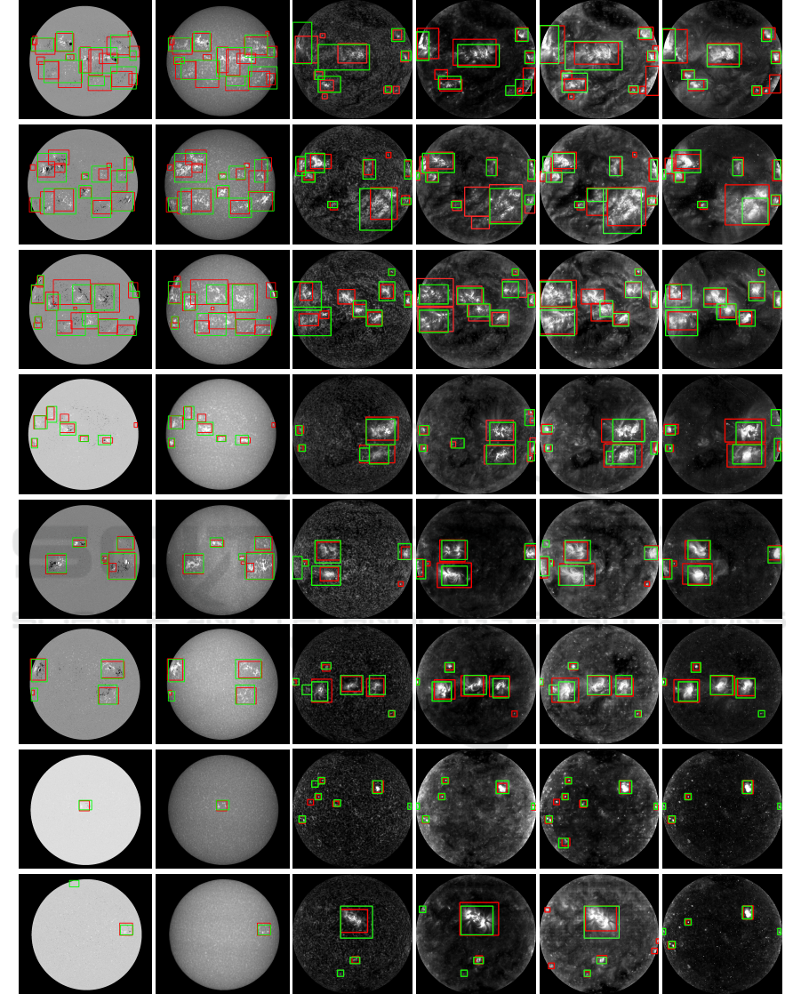
Figure 1: Ground-truth (red) and MSMT-CNN’s (green) detection of ARs in randomly selected images from (left to right)
SOHO/MDI Magnetogram and PM/SH 3934
˚
A, SOHO/EIT 304
˚
A, 171
˚
A, 195
˚
A, and 284
˚
A. Contrast has been increased
for convenience of visualisation.
ICPRAM 2021 - 10th International Conference on Pattern Recognition Applications and Methods
454

unique information. Our multi-tasking framework
aims at getting specialised results for each image
band, in contrast to most existing works where fo-
cus is on producing a unique prediction to all im-
age bands. This is crucial since the localisation in-
formation may differ from one band to another in so-
lar (sparse) multi-spectral images. Yet, all bands are
correlated, which motivates point 2. Our framework
exploits the inter-dependencies between the different
bands by its joint analysis strategy, increasing the ro-
bustness of its performance in individual bands.
Furthermore, our framework emulates how ex-
perts manually detect ARs (see also Section 3.1),
where a suspected region’s correlation with other
bands is evaluated prior to its final classification. This
demonstrates the usefulness and importance of ac-
counting for (spatially and temporally) neighbouring
slices in robustly detecting ARs.
The MSMT-CNN framework is very modular and
flexible. It may accommodate any number of avail-
able multi-spectral images. Additionally, since differ-
ent scenarios may require different fusion strategies
(as suggested by existing works), the modularity of
our framework allows it to be easily adapted to dif-
ferent types and levels of feature fusion (e.g. addi-
tion and concatenation, early and late). This modular
design also allows our framework to adopt different
backbone architectures (e.g. Faster RCNN in our ex-
periments). Indeed, its 3 key principles are applicable
to any backbone, as they are not architecture depen-
dent.
2.1 Pre-processing
The input of our system are time-matched observa-
tions, possibly acquired by different instruments or
at different orientations of the same instrument. As
such they need to be spatially aligned. We harmonise
the radius and center location of the solar disk, either
using SOHO image preparation routines, or through
Otsu thresholding of the solar disc of PM/SH images
followed by minimum enclosing circle fitting and re-
projection into a unified center and radius. Orienta-
tion is normalised by SOHO and PM routines to a
vertical north-south solar axis. Although this process
does not correct a possible small time difference and
resulting east-west rotation of the Sun between two
acquisitions, it ensures a sufficient alignment for our
purpose of AR detections from spatially (and tempo-
rally) correlated solar disks.
The SOHO/EIT images are prepared by EIT rou-
tines. We eliminate any prominences or solar erup-
tions by masking out all areas outside the solar disk.
The contrast of SOHO/MDI Magnetograms is en-
hanced by intensity rescaling. Contrast enhancement
was not used on SOHO/EIT and PM/SH images, as
it was found to have minimal effect on our detection
results.
Both datasets are augmented using north-south
flipping, east-west flipping, and a combination of the
two. Augmentation with arbitrary rotations of the
images is a popular way of augmenting astronomy
datasets. However, such rotations are ruled out from
our study because ARs tend to appear predominantly
alongside the solar equator.
Finally, a single-channel solar image was repeated
along the depth axis resulting in a 3-channel image in
order to match the pre-trained CNN’s input depth.
2.2 MSMT-CNN
Our detection DNN is presented in Fig. 2. A CNN
(ResNet50 or VGG16 in our experiments) is first used
as a feature extraction network. Parallel branches
(subnetworks) produce a feature map per image band,
following the late feature fusion strategy. This allows
the subnetworks’ filters to be optimised for their input
bands individually. The feature maps are then con-
catenated across the bands.
The combined feature map is jointly analysed by
one parallel module per image band that performs
Faster RCNN’s region proposal network (RPN). The
RPN stage uses three aspect ratios ([1:1], [1:2], [2:1])
and four sizes of anchor (32, 64, 128, and 256 pixel
width), found empirically to match well the typical
size and shape of ARs. One specialised RPN per im-
age band is trained.
At training, for each band, the correspondent re-
gion proposals along with the combined feature map
are used by a Faster RCNN’s detector module to per-
form the final prediction for the band. However, at
testing time, the band-specialised detector modules
use the region proposals from all bands. This com-
bination of region proposals helps finding potential
AR locations in bands where they are more difficult
to identify.
It is good to note that during training, the RPN’s
proposals for a band are filtered (i.e. labeled as pos-
itive or negative) with respect to their overlap with
the band’s ground-truth. Hence, combining them in
the training time would mean implicitly inheriting the
ground-truth of a band to another, in contradiction
with the band-specific ground-truth used for training
the detector module. This may hinder the learning of
both the RPN and detector modules. Therefore, re-
gion proposals are only combined at testing time to
ensure a better learning of the final detection modules.
Active Region Detection in Multi-spectral Solar Images
455
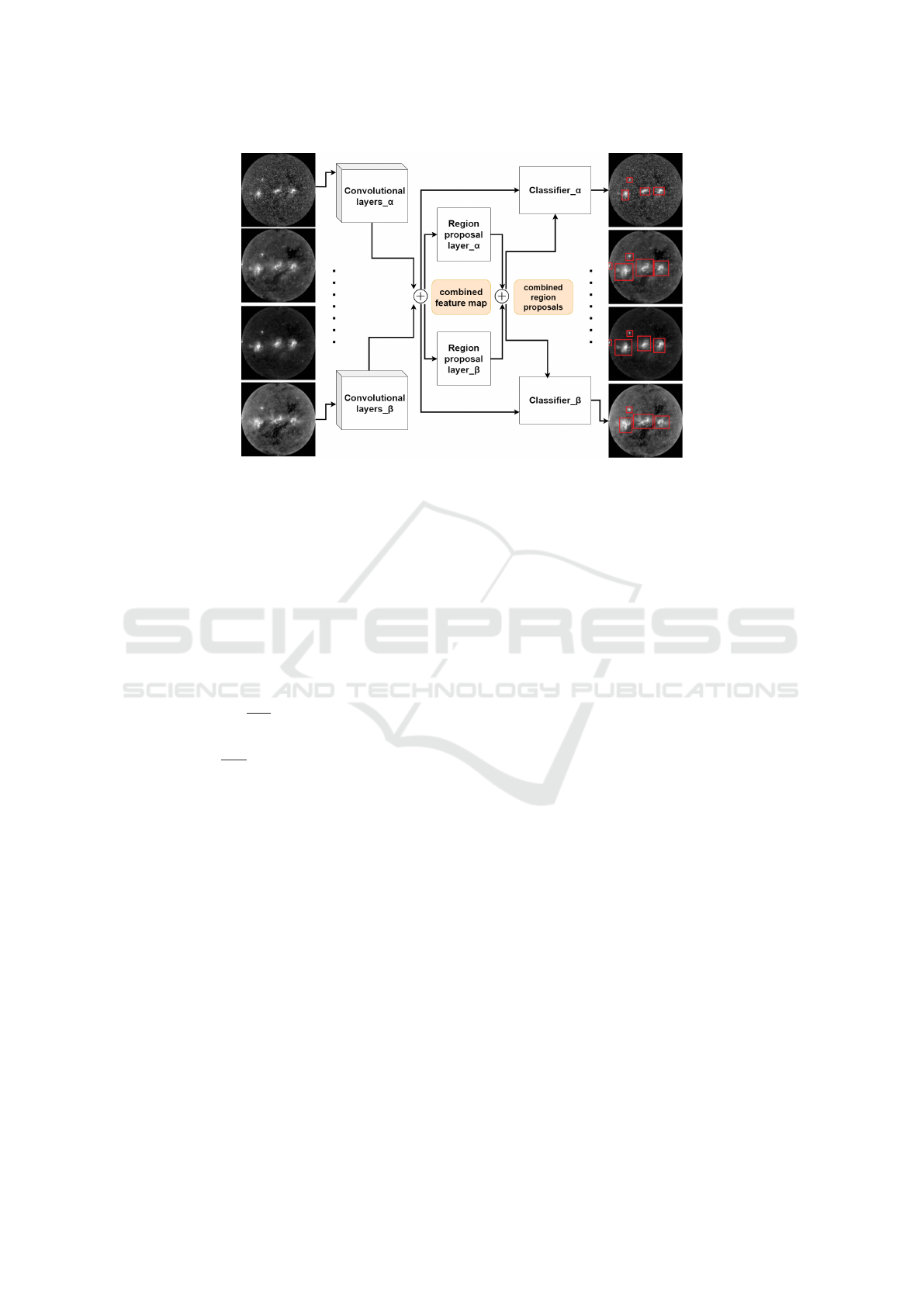
Figure 2: MSMT for detection using the Faster-RCNN backbone. ‘Plus’ sign denotes concatenation of the feature maps, or
of the lists of region proposals (at testing time).
Using the combined feature map for both RPN
prediction and classification helps the network learn
the relationship between the image bands and hence
provide more consistent region proposals and final
predictions. We demonstrate in Section 3 that this is
particularly helpful in cases where an AR is difficult
to detect in a single band.
The network is trained in the same way as the orig-
inal Faster RCNN, using all input bands and branches
according to a combined loss function:
L =
∑
b
1
N
cls
∑
i
L
cls
(p
b
i
, p
∗
b
i
)
+ λ
1
N
reg
∑
i
p
∗
b
i
L
reg
(t
b
i
, t
∗
b
i
)
(1)
where b and i refer to the image band and the
index of the bounding box being processed, respec-
tively. The terms L
cls
and L
reg
are the bounding-
box classification loss and the bounding-box regres-
sion loss defined in (Ren et al., 2015). N
cls
and N
reg
represent the size of the mini batch being processed
and the number of anchors, respectively. λ balances
the classification and the regression losses (we set λ
to 10 as suggested in (Ren et al., 2015)). p and p
?
are the predicted anchor’s class probability and its ac-
tual label, respectively. Lastly, t and t
?
represent the
predicted bounding box coordinates and the ground-
truth coordinates, respectively. It is worth noting that
our proposed framework is not limited to using Faster
RCNN’s loss and may be trained with using other
task-suitable loss functions.
During training, the weights of each stage (i.e.
feature extraction, region proposal, and detection)
are stored independently whenever the related Faster
RCNN loss decreases. At testing time, the best per-
forming set of weights is retrieved per stage. We re-
fer to this practice as ‘Multi-Objective Optimisation’
(MOO). The improved performance that we observe
in Section 3 may be explained by each stage having a
different objective to optimise, which may be reached
at different times.
In this paper, we experiment with a 2, 3, and 4-
band pipeline. However, the approach may generalise
straightforwardly to n bands and new imaging modal-
ities. Similarly, our framework may exploit any DNN
architecture, and may be updated with new state-of-
the-art DL architectures easily.
3 EXPERIMENTS
Our framework was implemented using Tensorflow
and run on an NVIDIA GeForce GTX 1080 Ti. We
evaluate our detection stage using precision, recall,
and F1-score. A detection is considered a true positive
if its intersection with a ground-truth box is greater or
equal to 50% of either the predicted or ground-truth
area. We empirically found that this provides a good
trade-off of precision over recall. Non maximum sup-
pression (NMS) is used to discard any redundant de-
tections.
All tested CNN were initialised with pre-trained
ImageNet weights. Indeed, we demonstrated in
(Crabbe et al., 2015) that CNNs pre-trained on RGB
images may fine-tune and adapt well to other modal-
ities such as depth images, provided that the im-
age’s gain and contrast are suitably enhanced to match
those of the pre-training RGB images.
ICPRAM 2021 - 10th International Conference on Pattern Recognition Applications and Methods
456

3.1 Data
We consider data from SOHO (space-based) and
PM observatory (ground-based). We use the bands
171
˚
A and 195
˚
A (transition region), 284
˚
A (corona),
and 304
˚
A (chromosphere and base of transition
region) from SOHO/EIT, 3934
˚
A (chromosphere)
from PM/SH, and line-of-sight magnetograms (pho-
tosphere) from SOHO/MDI, as illustrated in Fig. 1.
To account for the regular solar cycle, we select im-
ages evenly from each of 3 periods of varying solar
activity level, with years 2002-03, 2004-05, and 2008-
10 for high, medium, and low activity respectively.
We publish two new datasets with detection an-
notations (i.e bounding boxes): the Lower Atmo-
sphere Dataset (LAD) and Upper Atmosphere Dataset
(UAD). All annotations were validated by a solar
physics expert.
Localising ARs in multi-spectral images can be
challenging due to inconsistent numbers of polarity
centers, shapes, sizes, and activity levels. To miti-
gate this issue, when manually annotating, we exploit
neighboring image bands, magnetograms, as well as
temporal information where we examine the evolu-
tion of a suspected AR to validate its detection and
localisation. We designed a new multi-spectral label-
ing tool
2
which displays, side by side, images from an
auxiliary modality and from a sequence of 3 previous
and 3 subsequent time steps.
Table 1: Technical summary of the two annotated datasets.
# numbers are in train / test format.
Dataset Modality # images # boxes
UAD
SOHO/EIT 284
˚
A 283 / 40 2205 / 287
SOHO/EIT 171
˚
A 283 / 40 1919 / 262
SOHO/EIT 195
˚
A 283 / 40 2341 / 330
SOHO/EIT 304
˚
A 283 / 40 2016 / 263
LAD
PM/SH 3934
˚
A 213 / 53 1380 / 406
SOHO/MDI magn. 213 / 53 1380 / 406
Auxiliary imaging modalities may have different
observation frequencies and times, therefore we work
with time-matched images, i.e. the time-closest im-
age, if any, in a 12-hour window during which ARs
may not undergo any significant change.
ARs have a high spatial coherence in 3934
˚
A and
magnetogram images due to the physical proximity
of the two imaged regions. Hence, when annotating
3934
˚
A images, time-matched magnetograms were
used as an extra support. Furthermore, the 3934
˚
A
bounding boxes could be considered to be good ap-
proximations of magnetograms’ annotations. Table
2
Our labeling tool will be released on the project’s web-
site.
1 presents an overview of annotated images for both
datasets. We split the datasets into training and testing
as indicated in the table.
To compare against SPOCA, we consider a subset
of the UAD testing set for which SPOCA detection
results are available in HFC: the SPOCA subset. It
consists of 26 testing images (181, 168, 213, and 166
bounding boxes in the 304
˚
A, 171
˚
A, 195
˚
A and 284
˚
A
images respectively).
3.2 Independent Detection on Single
Image Bands
We first compare detection results of Faster RCNN
over individual image bands analysed independently
(Table 2). This aims to evaluate different feature ex-
traction DNNs, and will further serve as baseline to
assess our proposed framework.
The ResNet50 architecture consistently produces
better results than the VGG one with higher F1 scores
in all experiments. Based on these results, we adopt
the ResNet50 architecture as backbone for our frame-
work in the next experiments.
Table 2: Detection performance of the single image band
detectors. For each band, the highest scores are highlighted
in bold.
Detector Dataset Band Precision Recall F1
Faster
RCNN
(ResNet50)
LAD 3934
˚
A 0.93 0.82 0.87
LAD Magn. 0.89 0.78 0.83
UAD 304
˚
A 0.73 0.83 0.78
UAD 171
˚
A 0.84 0.89 0.86
UAD 195
˚
A 0.81 0.75 0.78
UAD 284
˚
A 0.86 0.82 0.84
SPOCA 304
˚
A 0.72 0.82 0.77
SPOCA 171
˚
A 0.87 0.87 0.87
SPOCA 195
˚
A 0.82 0.73 0.77
SPOCA 284
˚
A 0.86 0.82 0.84
Faster
RCNN
(VGG16)
UAD 304
˚
A 0.67 0.78 0.72
UAD 171
˚
A 0.84 0.81 0.82
UAD 195
˚
A 0.79 0.73 0.76
UAD 284
˚
A 0.83 0.81 0.82
SPOCA 304
˚
A 0.68 0.80 0.74
SPOCA 171
˚
A 0.85 0.80 0.82
SPOCA 195
˚
A 0.78 0.72 0.75
SPOCA 284
˚
A 0.84 0.82 0.83
When comparing the detection results per image
band, we notice that 304
˚
A images are repeatedly
amongst the most difficult to analyse in UAD, having
the lowest F1-scores in all tests. On the other hand,
171
˚
A has the best results of UAD bands, followed by
284
˚
A and 195
˚
A. This may be explained by ARs hav-
ing a denser or less ambiguous appearance in 171
˚
A,
195
˚
A, and 284
˚
A image bands than in 304
˚
A since
they are higher in the corona. A similar observation
can be made in the LAD dataset when comparing the
magnetogram results to 3934
˚
A, where magnetograms
Active Region Detection in Multi-spectral Solar Images
457

observe a lower altitude than 3934
˚
A.
We also notice a strong contrast between a same
detector’s precision and recall on the different UAD
bands. This further demonstrates that these bands are
not equal in how easily they may be analysed, even
though they were acquired at the same time with same
size and resolution.
Detections are visually verified to be poorer for
small ARs and for spread and faint ones with more
ambiguous boundaries. Visual inspection also con-
firms the different performances in various bands be-
ing caused by differing visual complexities of ARs.
These observations suggest that detecting ARs us-
ing information provided by a single band may be an
under-constrained problem.
3.3 Joint Detection on Multiple Image
Bands
We now present the results of our framework when
detecting ARs over the LAD/UAD bands jointly.
Joint detection results are summarised in Table 3.
We first experimented with different types of feature-
fusion (image-level and feature-level, by addition and
concatenation) over the LAD dataset.
Overall, the three approaches show an enhanced
performance in contrast to single band based detec-
tion. However, we find that late fusion with concate-
nation performs best. Hence, we pick this approach
for all following experiments.
We also evaluate the benefit of our MOO strat-
egy using our 2-band architecture over the UAD. This
approach generally improves the F1-scores in most
bands comparing to the non-MOO architectures. This
behaviour may indicate that the two feature extrac-
tion stages were indeed more effectively optimised for
their different tasks at different epochs. We retain this
MOO approach for all other experiments.
On the UAD dataset, with various combinations of
2 bands, we notice a general improvement over single
band detections. In addition, the performance varies
in correspondence to the bands being used. Combin-
ing bands that are difficult to analyse (304
˚
A or 195
˚
A
that have lowest F1-scores in the single band analy-
ses) with easier bands (171
˚
A and 284
˚
A) unsurpris-
ingly enhances their respective performance. More
interestingly, combining the difficult 304
˚
A and 195
˚
A
bands together also improve on their individual per-
formance. Similarly, when combining bands that are
easier to analyse (171
˚
A and 284
˚
A), in contrast to
using combinations of difficult and easy bands in the
analysis, performances are also improved over their
individual analyses. Following these settings, our 2-
band based approach was able to record higher or
similar F1-scores in contrast to the best performing
single-band detector. This supports our hypothesis
that joint detection may provide an increased robust-
ness through learning the inter-dependencies between
the image bands.
Table 3: AR detection performance of the MSMT-CNN de-
tectors. For each band, the highest scores are highlighted in
bold.
Detector Dataset Band Prec. Recall F1
MSMT (ResNet50
– MOO)
LAD
3934
˚
A 0.97 0.82 0.89
Magn. 0.96 0.85 0.90
MSMT
(ResNet50)
UAD
171
˚
A 0.92 0.77 0.84
284
˚
A 0.90 0.81 0.85
171
˚
A 0.82 0.85 0.83
195
˚
A 0.86 0.72 0.78
195
˚
A 0.88 0.67 0.77
284
˚
A 0.84 0.78 0.81
304
˚
A 0.82 0.79 0.80
195
˚
A 0.87 0.75 0.80
MSMT (ResNet50
– MOO)
UAD
171
˚
A 0.90 0.83 0.87
284
˚
A 0.93 0.80 0.86
SPOCA
171
˚
A 0.89 0.83 0.86
284
˚
A 0.92 0.80 0.86
UAD
171
˚
A 0.86 0.77 0.82
195
˚
A 0.89 0.75 0.81
SPOCA
171
˚
A 0.83 0.77 0.80
195
˚
A 0.86 0.73 0.79
UAD
195
˚
A 0.88 0.68 0.77
284
˚
A 0.84 0.78 0.81
SPOCA
195
˚
A 0.87 0.67 0.75
284
˚
A 0.81 0.78 0.80
UAD
304
˚
A 0.82 0.78 0.80
195
˚
A 0.88 0.78 0.83
SPOCA
304
˚
A 0.79 0.78 0.79
195
˚
A 0.85 0.77 0.81
UAD
304
˚
A 0.78 0.74 0.76
171
˚
A 0.76 0.76 0.76
284
˚
A 0.79 0.78 0.78
UAD
304
˚
A 0.93 0.69 0.79
171
˚
A 0.94 0.66 0.78
195
˚
A 0.91 0.72 0.80
284
˚
A 0.93 0.66 0.77
MSMT (ResNet50
– MOO)
Combining
neighbour bands
UAD
304
˚
A 0.72 0.76 0.74
171
˚
A 0.74 0.79 0.76
195
˚
A 0.81 0.73 0.77
284
˚
A 0.68 0.84 0.75
SPOCA SPOCA
171
˚
A 0.54 0.93 0.68
195
˚
A 0.58 0.82 0.68
(Jarolim et al.,
2019) using Faster
RCNN (ResNet50)
UAD
304
˚
A 0.73 0.83 0.78
171
˚
A 0.80 0.90 0.84
195
˚
A 0.83 0.72 0.77
284
˚
A 0.86 0.80 0.83
Moreover, the most dramatic improvement in F1-
scores across both LAD and UAD datasets is for the
3934
˚
A images when magnetograms are added to the
analysis. This is in line with the current understanding
of AR having strong magnetic signatures.
Generally, in the UAD dataset, we find that us-
ing a combination of 2 bands produces the best re-
sults in comparison to using 3 or 4 bands. This may
be caused by the fact that optimising the network for
ICPRAM 2021 - 10th International Conference on Pattern Recognition Applications and Methods
458

multiple tasks (2, 3, or 4 detection tasks) simultane-
ously increases the complexity of the problem. While
the network successfully learned to produce better de-
tections in the case of 2 bands, it was difficult to find a
generalised yet optimal model for 3 or 4 bands at the
same time.
Furthermore, since bands imaging consecutive
layers of solar atmosphere are expected to be highly
correlated, we test our framework by combining di-
rectly neighbouring bands together, such that a pre-
diction for a band is performed using the band’s own
feature map combined with the feature map(s) of its
available (1 or 2) direct neighbour(s). This approach
gets the highest recall score on the UAD band 284
˚
A
of all tests, where it is combined with the 195
˚
A band.
However, it does not improve the performance on the
other bands comparing to the single-band and 2-band
based experiments.
We compare against state-of-the-art SPOCA (Ver-
beeck et al., 2013) on the SPOCA subset, and against
the first stage of (Jarolim et al., 2019) (sequentially
fine-tuned networks) by adapting their approach to
Faster RCNN and testing it on UAD. SPOCA de-
tections were obtained from 171
˚
A and 195
˚
A im-
ages only, combined as two channels of an RGB im-
age, and SPOCA produces a single detection for both
bands. We compare this detection against the ground
truth of each of the bands individually. To prove the
robustness and versatility of our detector, we also ex-
periment with a combination of chromosphere, tran-
sition region, and corona bands on the SPOCA subset
in addition to the whole UAD.
On the SPOCA subset, over the bands 171
˚
A and
195
˚
A for which it is designed, SPOCA gets the poor-
est performance of all multi-band and single-band ex-
periments. It is worth noting that this method relies
on manually tuned parameters according to the devel-
opers’ own definition and interpretation of AR bound-
aries, which may differ from the ones we used when
annotating the dataset. While supervised DL-based
methods could integrate this definition during train-
ing, SPOCA could not perform such adaptation. This
may have had a negative impact on its scores. Fur-
thermore, visual inspection shows a poor performance
for SPOCA on low solar activity images. This may
be due to the use of clustering in SPOCA, since in
low activity periods the number of AR pixels (if any)
is significantly smaller than solar background pixels,
which makes it hard to identify clusters.
Moreover, the fine-tuned networks of (Jarolim
et al., 2019) suffer from a high rate of false positives,
and show a close performance to single band detec-
tion using Faster RCNN with an identical precision,
recall and F1-score over the band 304
˚
A and a slight
decrease over the other 3 bands. This may be due
to the fact that its transfer learning does not incor-
porate the inter-dependencies directly when analysing
the different bands.
4 CONCLUSION
We presented MSMT-CNN, a multi-branch and multi-
tasking framework to tackle the 3D solar AR detec-
tion problem from multi-spectral images that observe
different cuts of the 3D solar atmosphere. MSMT-
CNN analyses multiple image bands jointly to pro-
duce consistent detection across them. It is a flexi-
ble framework that may use any CNN backbone, and
may be be straightforwardly generalised to any num-
ber and modalities of images. MSMT-CNN showed
competitive results against baseline and state-of-the-
art detection methods.
REFERENCES
Benkhalil, A., Zharkova, V., Zharkov, S., and Ipson, S.
(2006). Active region detection and verification with
the solar feature catalogue. Solar Phys.
Crabbe, B., Paiement, A., Hannuna, S., and Mirmehdi,
M. (2015). Skeleton-free body pose estimation from
depth images for movement analysis. In ICCVW.
Guo, Z., Li, X., Huang, H., Guo, N., and Li, Q. (2019).
Deep learning-based image segmentation on multi-
modal medical imaging. IEEE TRPMS.
Ishii, T., Simo-Serra, E., Iizuka, S., Mochizuki, Y., Sug-
imoto, A., Ishikawa, H., and Nakamura, R. (2016).
Detection by classification of buildings in multispec-
tral satellite imagery. In ICPR.
Jarolim, R., Veronig, A., Hofmeister, S., Temmer, M.,
Heinemann, S., Podladchikova, T., and Dissauer, K.
(2019). Multi-channel coronal hole detection with a
CNN. In ML-Helio.
Mohajerani, S. and Saeedi, P. (2019). Cloud-Net: An end-
to-end cloud detection algorithm for Landsat 8 im-
agery. In IGARSS.
Ren, S., He, K., Girshick, R., and Sun, J. (2015). Faster R-
CNN: Towards real-time object detection with region
proposal networks. In NIPS.
Revathy, K., Lekshmi, S., and Prabhakaran Nayar, S.
(2005). Fractal-based fuzzy technique for detection
of active regions from solar images. Solar Phys.
Verbeeck, C., Delouille, V., Mampaey, B., and Visscher,
R. D. (2013). The SPoCA-suite: Software for extrac-
tion, characterization, and tracking of active regions
and coronal holes on EUV images. Astron. Astrophys.
Wagner, J., Fischer, V., Herman, M., and Behnke, S. (2016).
Multispectral pedestrian detection using deep fusion
convolutional neural networks. In ESANN.
Active Region Detection in Multi-spectral Solar Images
459
