
LongiControl: A Reinforcement Learning Environment for Longitudinal
Vehicle Control
Jan Dohmen, Roman Liessner, Christoph Friebel and Bernard B
¨
aker
Dresden Institute of Automobile Engineering, TU Dresden, George-B
¨
ahr-Straße 1c, 01069 Dresden, Germany
Keywords:
Reinforcement Learning, Artificial Intelligence, Deep Learning, Machine Learning, Autonomous Driving,
Longitudinal Control, OpenAI Gym.
Abstract:
Reinforcement Learning (RL) might be very promising for solving a variety of challenges in the field of
autonomous driving due to its ability to find long-term oriented solutions in complex decision scenarios. For
training and validation of a RL algorithm, a simulative environment is advantageous due to risk reduction
and saving of resources. This contribution presents an RL environment designed for the optimization of
longitudinal control. The focus is on providing an illustrative and comprehensible example for a continuous
real-world problem. The environment will be published following the OpenAI Gym interface, allowing for
easy testing and comparing of novel RL algorithms. In addition to details on implementation reference is also
made to areas where research is required.
1 INTRODUCTION
A large proportion of road traffic accidents are due to
human error (Gr
¨
undl, 2005). Autonomous vehicles
and driver assistance systems are therefore promising
ways to increase road safety in the future (Bertoncello
and Wee, 2015). Moreover, global climate change and
dwindling resources are increasingly contributing to
raising society’s awareness of environmental policy
issues. In addition to vehicle electrification, advanc-
ing automation in transport promises a much more ef-
ficient use of energy. Assistance systems in particular
which support the predictive longitudinal control of a
vehicle can lead to significant energy savings (Radke,
2013).
A commonly chosen approach for energy-efficient
optimization of the longitudinal control is based on
the use of dynamic programming. Although this is ba-
sically capable of finding the discrete global optimum
it requires in advance a comprehensive problem mod-
eling, a deterministic environment and a discretiza-
tion of the action space. Especially when considering
other road users the conventional approaches there-
fore reach their limits (Ye et al., 2017). A priori, ar-
bitrary traffic cannot be sufficiently modeled and thus
no precise knowledge of the entire route can be given.
Furthermore, the computing power available in the
vehicle is not sufficient to perform new optimizations
depending on the constantly changing environment.
Online use in the vehicle is therefore unlikely.
The developments in the field of machine learn-
ing, especially deep reinforcement learning (DRL),
are very promising. The learning system recognizes
the relations between its actions and the associated
effect on the environment. This enables the system
to react immediately to environmental influences in-
stead of just following a previously calculated plan.
After proving in recent years to solve challenging
video games (Mnih et al., 2013) on a partly superhu-
man level DRL has lately been increasingly used for
engineering and physical tasks (Hinssen and Abbeel,
2018). Examples are the cooling of data centers (Gao,
2014), robotics (Gu et al., 2016), the energy manage-
ment of hybrid vehicles (Liessner et al., 2018) or self-
driving vehicles (Kendall et al., 2018) (Sallab et al.,
2017). This motivates to apply such an approach also
to the problem of optimizing longitudinal control.
In this contribution we propose LongiControl
(Dohmen et al., 2019), a RL environment being
adapted to the OpenAI Gym standardization. Even
though LongiControl could be regarded as another
simplified solution to the longitudinal control prob-
lem, the main focus, however, is rather to provide a
stochastic and continuous RL environment being de-
signed in such a way that RL agents can be trained
with an ordinary notebook in a relatively short pe-
riod of time. Furthermore, the longitudinal con-
trol problem has several easily comprehensible chal-
1030
Dohmen, J., Liessner, R., Friebel, C. and Bäker, B.
LongiControl: A Reinforcement Learning Environment for Longitudinal Vehicle Control.
DOI: 10.5220/0010305210301037
In Proceedings of the 13th International Conference on Agents and Artificial Intelligence (ICAART 2021) - Volume 2, pages 1030-1037
ISBN: 978-989-758-484-8
Copyright
c
2021 by SCITEPRESS – Science and Technology Publications, Lda. All rights reserved

lenges making it a suitable example to test and com-
pare novel RL algorithms while also providing the
possibility to investigate advanced topics like multi-
objective RL (trade-off between conflicting goals of
travel time minimization and energy consumption),
safe RL (violation of speed limits may lead to acci-
dents) or explainable RL (easy-to-follow actions and
states). We aim to bridge real-world motivated RL
with easy accessibility inside a highly relevant prob-
lem.
This publication is structured as follows. In sec-
tion 2 overviews are given on the longitudinal control
problem and on the basic principles of RL. In section
3 we present the LongiControl environment describ-
ing the route simulation, the vehicle model and its in-
teraction with a RL agent. Thereafter, in section 4 we
show exemplary results for different training phases
and give a brief insight into the challenges with con-
trary reward formulations. This is followed by the
conclusion in section 5 providing a basis for future
working directions.
2 BACKGROUND
2.1 Longitudinal Control
Energy-Efficient Driving. In general terms, an en-
ergetically optimal driving corresponds to a global
minimization of the input energy E in the interval
t
0
≤ t ≤ T as a function of acceleration a, velocity
v and power P:
E =
Z
T
t
0
P(t,a(t),v(t))dt (1)
At the same time, according to external requirements,
such as other road users or speed limits, the following
boundary conditions must be met:
v
lim,min
(x) ≤ v ≤ v
lim,max
(x)
a
lim,min
(v) ≤ a ≤ a
lim,max
(v)
˙a
lim,min
(v) ≤ ˙a ≤ ˙a
lim,max
(v) .
(2)
Where v is the velocity, a is the acceleration and ˙a is
the jerk, with (·)
lim,min
and (·)
lim,max
representing the
lower and upper limits respectively.
Following Freuer (Freuer, 2015) the optimization
can be divided roughly into four areas:
1. optimization of the vehicle properties,
2. optimization of traffic routing,
3. optimization on an organizational level,
4. optimization of vehicle control.
This paper deals with the last point. In various contri-
butions (Barkenbus, 2010) (Uebel, 2018) an adapted
vehicle control system is assigned an enormous sav-
ings potential. In addition to the safety aspect, as-
sistance systems supporting vehicle control are be-
coming increasingly important for this reason as well.
This trend is made possible by comprehensive sensor
technology and the supply of up-to-date route data.
In terms of longitudinal control, energy-saving driv-
ing modes can thus be encouraged:
• driving in energy-efficient speed ranges,
• keeping an appropriate distances to vehicles in
front,
• anticipatory deceleration and acceleration.
Simulation. Simulations become more and more
important in automotive engineering. According to
Winner et al. (Winner and Wachenfeld, 2015), in the
context of the automotive industry the overall system
is composed of three parts: the vehicle, the driving en-
vironment and the vehicle control. These three com-
ponents interact through an exchange of information
and energy.
Within the simulation a vehicle model is needed
which indicates the energy consumption. In general,
physical and data-based approaches are suitable for
modeling those (Isermann, 2008).
External influences are represented by the driving
environment. This includes for example information
about other road users and route data such as traffic
light signals or speed limits. These information are
used then by the vehicle control as boundary condi-
tions for the driving strategy.
While in reality with increasing automation the in-
formation content of the sensor system in vehicles is
increasing (Winner et al., 2015), this information can
be easily generated in the simulation. Considering
the modeling of the driving environment a distinction
must be made between deterministic and stochastic
approaches. In the deterministic case it is assumed
that the driving environment behaves the same in ev-
ery run. Changes during the simulation are not al-
lowed. This means that reality can only be repre-
sented in a very simplified way. For example a sudden
change of a traffic light signal or an unforeseen brak-
ing of the vehicle in front is not represented by such
a model. In contrast, the stochastic approach offers
the possibility to vary external influences during the
simulation. Therefore, this type of modeling is much
closer to the real driving situation.
Optimization. The aim of the RL environment is
to train an agent to drive an electric vehicle a single-
LongiControl: A Reinforcement Learning Environment for Longitudinal Vehicle Control
1031

lane route as energy-efficient as possible. This cor-
responds to the minimization of Equation 1 while
considering the corresponding boundary conditions in
Equation 2.
Examples for state-of-the-art approaches for the
optimization of the longitudinal control problem are
Dynamic Programming (Bellman, 1954), Pontrya-
gin’s Maximum Principle (Pontryagin et al., 1962) or
a combination of both (Uebel, 2018). As previously
mentioned these approaches have two basic limita-
tions: they are based on deterministic models and suf-
fer from the curse of dimensionality.
According to (Sutton and Barto, 2018) and (Bert-
sekas and Tsitsiklis, 1999) RL approaches are a so-
lution to this dilemma. The main difference between
Dynamic Programming and RL is that the former as-
sumes to know the complete model. RL approaches
on the other hand only require the possibility of inter-
action with the environment model. Without knowing
its inner structure solutions are learned. In modern
deep RL (DRL), the use of neural networks for func-
tion approximation also allows to handle continuous
state spaces and react to previously unknown states.
2.2 Reinforcement Learning
A standard reinforcement learning framework is con-
sidered, consisting of an agent that interacts with an
environment (see Figure 1). The agent perceives its
state s
t
∈ S in the environment in each time step t =
0,1,2,... and consequently chooses an action a
t
∈ A.
With this, the agent in turn directly influences the en-
vironment resulting in an updated state s
t+1
for the
next time step. The selected action is evaluated using
a numerical reward r
t+1
(s,a). The sets S and A con-
tain all possible states and actions that can occur in
the description of the problem to be learned.
The policy π(a | s) specifies for each time step
which action is to be executed depending on the state.
The aim is to select actions in such a way that the cu-
mulative reward is maximized.
Policy gradient methods are probably the most
popular class of RL algorithms for continuous prob-
lems. Currently very relevant examples for such
methods are Proximal Policy Optimization (PPO)
(Schulman et al., 2017), Deep Deterministic Pol-
icy Gradient (DDPG) (Lillicrap et al., 2015) or Soft
Actor-Critic (SAC) (Haarnoja et al., 2018).
Agent
Environment
State,
Reward
Action
Figure 1: Agent environment interaction.
3 RL ENVIRONMENT
3.1 OpenAI Gym
OpenAI Gym (Brockman et al., 2016) is a widely
used open-source framework with a large number
of well-designed environments to compare RL algo-
rithms. It does not rely on a specific agent structure
or deep learning framework. To provide an easy start-
ing point for RL and the longitudinal control problem,
the implementation of the LongiControl environment
follows the OpenAI Gym standardization.
3.2 Route Simulation
Figure 2 shows an example of the simplified track im-
plementation within the simulation.
50 70 90
Figure 2: An example for the track visualization.
Equation of Motion. The vehicle motion is mod-
eled simplified as uniform accelerated. The simula-
tion is based on a time discretization of ∆t = 0.1 s.
The current velocity v
t
and position x
t
are calculated
as follows:
v
t
= a
t
∆t +v
t−1
x
t
=
1
2
a
t
(∆t)
2
+ v
t−1
∆t +x
t−1
The acceleration a
t
must be specified through the
agents action in each time step t. Since only the longi-
tudinal control is considered the track can be modeled
single-laned. Therefore, one-dimensional velocities
v
t
and positions x
t
are sufficient at this point.
ICAART 2021 - 13th International Conference on Agents and Artificial Intelligence
1032

Stochastic Route Modeling. The route simulation
is modeled in such a way that the track length may be
arbitrarily long and that arbitrarily positioned speed
limits specify an arbitrary permissible velocity. Here,
it is argued that this can be considered equivalent to a
stochastically modeled traffic.
Under the requirement that a certain safety dis-
tance to the vehicle in front must be maintained other
road users are simply treated as further speed limits
which depend directly on the distance and the differ-
ence in speed. For each time step the relevant speed
limit is then equal to the minimum of the distance-
related and traffic-related limit.
Restrictively, speed limits are generated
in a minimum possible distance of 100 m.
The permissible velocities are sampled from
[20, 30, 40, 50, 60, 70, 80, 90, 100 km/h] while
the difference of contiguous limits may not
be greater than 40 km/h. It should there-
fore apply x
lim, j+1
− x
lim, j
≥ 100 m and
|v
lim, j+1
− v
lim, j
| ≤ 40 km/h. The former is a
good compromise to induce as many speed changes
per trajectory as possible and to be able to identify
anticipatory driving at the same time. The second is
introduced as another simplification to speed up the
learning process. Very large speed changes may be
very hard for the agent to handle.
Up to 150 m in advance, the agent receives infor-
mation about the upcoming two speed limits.
3.3 Vehicle Model
Figure 3: Assigning the action to an acceleration.
The vehicle model derived from vehicle measurement
data (see figure 3) consists of several subcomponents.
These have the function of receiving the action of the
agent, assigning a physical acceleration value and out-
putting the corresponding energy consumption.
Assigning the Action to an Acceleration. The ac-
tion of the agent is interpreted in this environment as
the actuation of the vehicle pedals. In this sense, a
positive action actuates the accelerator pedal. A neg-
ative analogous action actuates the brake pedal. The
vehicle acceleration resulting from the pedal interac-
tion depends on the current vehicle speed (road slopes
are neglected) due to the limited vehicle motorization.
If neither pedal is actuated (corresponds to
action = 0), the vehicle decelerates its speed by simu-
lating the driving resistance. This means that to main-
tain a positive speed a positive action must be se-
lected.
It becomes clear from the explanations that three
speed-dependent acceleration values determine the
physical range of the agent. These are the maximum
and minimum acceleration and the acceleration value
for action = 0.
Determination of the Acceleration Values. The
speed-dependent maximum and minimum accelera-
tion can be determined from the measurement data
and the technical data of the vehicle. In the RL en-
vironment, the maximum and minimum values for
each speed are stored as characteristic curves. The
resulting acceleration at action = 0 is calculated phys-
ically. Using the driving resistance equation and the
vehicle parameters an acceleration value is calculated
for each speed. This is stored in the environment as
a speed-dependent characteristic curve, analogous to
the other two acceleration values.
Once the action, the current vehicle speed and the
three acceleration values are available the resulting
acceleration can be calculated as follows:
a
t
=
(a
max
− a
0
) · action + a
0
if action > 0
a
0
if action = 0
−(a
min
− a
0
) · action + a
0
if action < 0
Calculation of Energy Consumption. Knowing
the vehicle speed and acceleration the energy con-
sumption can be estimated from these two values. For
this purpose measured values of an electric vehicle
(Argonne National Laboratory, 2013) were learned
using a neural network and the network was stored
in the environment.
3.4 Agent Environment Interaction
In accordance with the basic principle of RL an agent
interacts with its environment through its actions and
receives an updated state and reward.
Action. The agent selects an action in the value
range [-1,1]. The agent can thus choose between a
LongiControl: A Reinforcement Learning Environment for Longitudinal Vehicle Control
1033

condition-dependent maximum and minimum accel-
eration of the vehicle. This type of modeling results
in the agent only being able to select valid actions.
State. The features of the state must provide the
agent with all the necessary information to enable a
goal-oriented learning process. The individual fea-
tures and their meaning are listed in Table 1.
When training neural networks the learning pro-
cess often benefits from the fact that the dimensions
of the input variables do not differ greatly from one
another. According to Ioffe et al. (Ioffe and Szegedy,
2015) the gradient descent algorithm converges faster
if the individual features have the same order of mag-
nitude. Since according to Table 1 different physical
quantities with different value ranges enter the state
a measure for normalization seems to be reasonable
at this point. All features are scaled min-max for this
purpose so that they are always in the fixed interval
[0, 1].
Table 1: Meaning of state features.
Feature Meaning
v(t) Vehicles’s current velocity
a
prev
(t) Vehicle acceleration of the last time
step, s.t. the agent is able to have an
intuition for the jerk
v
lim
(t) Current speed limit
v
v
v
lim, f ut
(t) The next two speed limit changes, as
long as they are within a range of
150 m
d
d
d
v
lim, f ut
(t) Distances to the next two speed limit
changes, as long as they are within a
range of 150 m
Reward. In the following, the reward function that
combines several objectives is presented. The expla-
nations indicate the complexity of the multi-objective
manner. The LongiControl Environment thus pro-
vides a good basis for investigating these issues and
for developing automated solutions to solve them.
A reward function defines the feedback the agent
receives for each action and is the only way to control
the agent’s behavior. It is one of the most important
and challenging components of an RL environment.
If only the energy consumption were rewarded (nega-
tively) the vehicle would simply stand still. The agent
would learn that from the point of view of energy con-
sumption it is most efficient simply not to drive. Al-
though this is true we still want the agent to drive in
our environment. So we need a reward that makes
driving more appealing to the agent. By comparing
different approaches the difference between the cur-
rent speed and the current speed limit has proven to
be particularly suitable. By minimizing the difference
the agent automatically sets itself in motion. In order
to still take energy consumption into account the re-
ward component is maintained with energy consump-
tion. A third reward component is caused by the jerk.
This is because our autonomous vehicle should also
be able to drive comfortably. To punish finally also
the violation of the speed limits a fourth reward part
is supplemented. Since RL is designed for a scalar
reward it is necessary to weight these four parts.
A suitable weighting is not trivial and poses a
great challenge. For the combined reward we propose
the following (see also Table 2):
r
t
= − ξ
f orward
r
f orward
(t)
− ξ
energy
r
energy
(t)
− ξ
jerk
r
jerk
(t)
− ξ
sa f e
r
sa f e
(t) ,
while
r
f orward
(t) =
|v(t) − v
lim
(t)|
v
lim
(t)
r
energy
(t) =
ˆ
E
r
jerk
(t) =
|a(t) − a
prev
(t)|
∆t
r
sa f e
(t) =
(
0 v(t) ≤ v
lim
(t)
1 v(t) > v
lim
(t)
.
ξ are the weighting parameters for all reward shares.
In some cases, the terms are used as penalty so that the
learning algorithm minimizes their amount. To make
it easier to get started with the environment we have
preconfigured a functioning weighting (see Table 3).
In the next section we will show some examples of
the effects of different weightings.
Table 2: Meaning of reward terms.
Reward Meaning
r
f orward
(t) Penalty for slow driving
r
energy
(t) Penalty for energy consumption
r
jerk
(t) Penalty for jerk
r
sa f e
(t) Penalty for speeding
4 EXAMPLES
In the following various examples of the environment
are presented. For training the agent is confronted
ICAART 2021 - 13th International Conference on Agents and Artificial Intelligence
1034
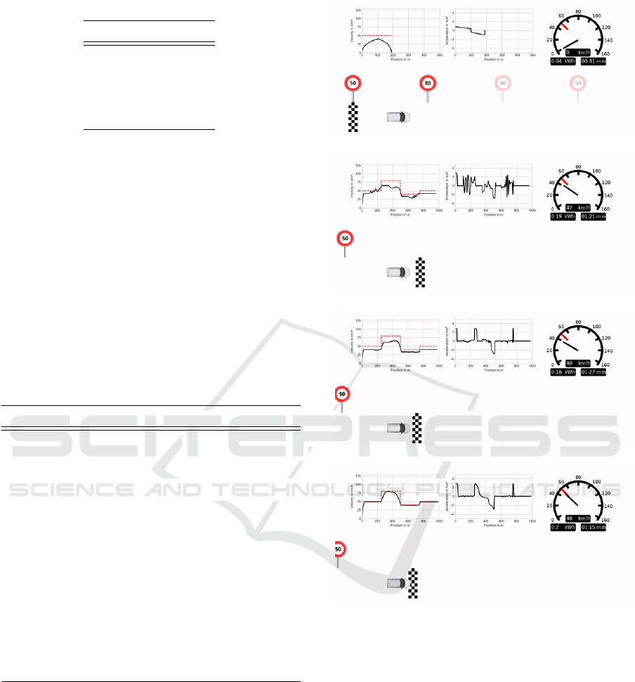
Table 3: Weighting parameters for the reward.
Parameter Value
ξ
f orward
(t) 1.0
ξ
energy
(t) 0.5
ξ
jerk
(t) 1.0
ξ
sa f e
(t) 1.0
with new routes in each run using the stochastic mode
of the environment. For validation it is always used
the same deterministic route to compare like with like.
4.1 Learning Progress
In the following different stages of an exemplary
learning process are presented. An implementation of
SAC (Haarnoja et al., 2018) was chosen as the deep
RL algorithm. The used hyperparameters are listed
in Table 4. Animated visualizations for the upcom-
ing learning stages can be found on GitHub (Dohmen
et al., 2019).
Table 4: SAC hyperparameter.
Parameter Value
optimizer Adam
learning rate 0.001
discount γ 0.99
replay buffer size 1000000
number of hidden layers (all networks) 2
number of hidden units per layer 64
optimization batch size 256
target entropy −dim(A)
activation function ReLU
soft update factor τ 0.01
target update interval 1
gradient steps 1
Beginning of the Learning Process. At the very
beginning of the learning process the agent remains
in place and does not move at all. Then after a few
more training epochs the agent starts to move but is
not yet able to finish the track. Figure 4a shows this
stage in the deterministic validation run.
After Some Learning Progress. After some
progress the agent is able to complete the course (see
Figure 4b) but ignores speed limits while driving very
(a) Beginning of the learning process.
(b) After some learning progress.
(c) After a longer training procedure.
(d) After an even longer training period.
Figure 4: Learning progress.
jerky. Obviously, this is not desirable. Therefore the
training continuous.
After a Longer Training Procedure. By letting the
agent train even longer it learns to drive more com-
fortably and finally starts to respect the speed limits
by an early enough deceleration. Though, in general
it is driving quite slow in relation to the maximum al-
lowed (see Figure 4c).
After an Even Longer Training Period. Finally
after an even longer training, it drives very smooth,
respects the speed limits while minimizing the safety
LongiControl: A Reinforcement Learning Environment for Longitudinal Vehicle Control
1035
margin to the maximum allowed (see Figure 4d).
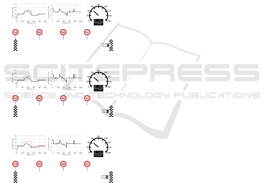
4.2 Multi-objective Optimization
As mentioned before, this problem has several con-
trary objectives. Thus also multi-objective investiga-
tions can be carried out. For a better understanding
we present three examples.
Reward Example 1. If only the movement reward
– the deviation from the allowed speed – is applied
(reward weighting [ξ
f orward
(t) = 1, ξ
energy
(t) = 0,
ξ
jerk
(t) = 0, ξ
sa f e
(t) = 0]) the agent violates the speed
limits because being 5 km/h too fast is rewarded the
same as being 5 km/h too slow (see Figure 5a).
(a) ξ
f orward
(t) = 1, ξ
energy
(t) = 0, ξ
jerk
(t) = 0,
ξ
sa f e
(t) = 0.
(b) ξ
f orward
(t) = 1, ξ
energy
(t) = 0, ξ
jerk
(t) = 0,
ξ
sa f e
(t) = 1.
(c) ξ
f orward
(t) = 1, ξ
energy
(t) = 0.5, ξ
jerk
(t) = 1,
ξ
sa f e
(t) = 1.
Figure 5: Reward weighting.
Reward Example 2. In the second example, the
penalty for exceeding the speed limit is added (reward
weighting [ξ
f orward
(t) = 1, ξ
energy
(t) = 0, ξ
jerk
(t) =
0, ξ
sa f e
(t) = 1]). This results in the agent actually
complying with the limits (see Figure 5b).
Reward Example 3. In the third example we
add the energy and jerk reward (reward weight-
ing [ξ
f orward
(t) = 1, ξ
energy
(t) = 0.5, ξ
jerk
(t) = 1,
ξ
sa f e
(t) = 1]). This results in the agent driving more
energy-efficiently and also choosing smoother accel-
erations (see Figure 5c).
These examples illustrate that the environment
provides a basis to investigate multi-objective op-
timization algorithms. For such investigations the
weights of the individual rewards can be used as con-
trol variables and the travel time, energy consumption
and the number of speed limit violations can be used
to evaluate the higher-level objectives.
5 CONCLUSION
By means of the proposed RL environment, which is
being adapted to the OpenAI Gym interface, we show
that it is easy to prototype and implement state-of-
art RL algorithms. The LongiControl environment
is suitable for various examinations: In addition to
the comparison of RL algorithms for continuous and
stochastic problems, LongiControl provides an exam-
ple for investigations in the area of multi-objective
RL, explainable RL and safe RL. Regarding the lon-
gitudinal control problem itself, further possible re-
search objectives may be among others the compar-
ison with planning algorithms for known routes and
the consideration of very long-term objectives like ar-
riving at a specific time.
LongiControl is designed to enable the commu-
nity to leverage the latest strategies of reinforce-
ment learning to address a real-world and high-impact
problem in the field of autonomous driving.
REFERENCES
Argonne National Laboratory (2013). Downloadable
dynamometer database (d3) generated at the ad-
vanced mobility technology laboratory (amtl) un-
der the funding and guidance of the u.s. depart-
ment of energy (doe). https://www.anl.gov/es/
downloadable-dynamometer-database.
Barkenbus, J. N. (2010). Eco-driving: an overlooked cli-
mate change initiative. Energy Policy, 38. https:
//doi.org/10.1016/j.enpol.2009.10.021.
Bellman, R. (1954). The theory of dynamic program-
ming. Bull. Amer. Math. Soc., 60(6):503–515. https:
//projecteuclid.org:443/euclid.bams/1183519147.
Bertoncello, M. and Wee, D. (2015). Mckinsey: Ten
ways autonomous driving could redefine the
automotive world. https://www.mckinsey.com/
industries/automotive-and-assembly/our-insights/
ICAART 2021 - 13th International Conference on Agents and Artificial Intelligence
1036

ten-ways-autonomous-driving-could-redefine-the/
-automotive-world.
Bertsekas, D. P. and Tsitsiklis, J. N. (1999). Neuro-dynamic
programming. 2te edition.
Brockman, G., Cheung, V., Pettersson, L., Schneider, J.,
Schulman, J., Tang, J., and Zaremba, W. (2016). Ope-
nai gym. CoRR, abs/1606.01540. http://arxiv.org/abs/
1606.01540.
Dohmen, J., Liessner, R., Friebel, C., and B
¨
aker, B. (2019).
LongiControl environment for OpenAI gym. https:
//github.com/dynamik1703/gym-longicontrol.
Freuer, A. (2015). Ein Assistenzsystem f
¨
ur die energetisch
optimierte L
¨
angsf
¨
uhrung eines Elektrofahrzeugs. PhD
thesis.
Gao, J. (2014). Machine learning applications for data cen-
ter optimization.
Gr
¨
undl, M. (2005). Fehler und Fehlverhalten als Ur-
sache von Verkehrsunf
¨
allen und Konsequenzen f
¨
ur
das Unfallvermeidungspotenzial und die Gestaltung
von Fahrerassistenzsystemen. PhD thesis, University
Regensburg.
Gu, S., Lillicrap, T. P., Ghahramani, Z., Turner, R. E.,
and Levine, S. (2016). Q-prop: Sample-efficient
policy gradient with an off-policy critic. CoRR,
abs/1611.02247. http://arxiv.org/abs/1611.02247.
Haarnoja, T., Zhou, A., Hartikainen, K., Tucker, G., Ha,
S., Tan, J., Kumar, V., Zhu, H., Gupta, A., Abbeel, P.,
and Levine, S. (2018). Soft actor-critic algorithms and
applications. CoRR, abs/1812.05905. http://arxiv.org/
abs/1812.05905.
Hinssen, P. and Abbeel, P. (2018). Everything is going
to be touched by ai. https://nexxworks.com/blog/
everything-is-going-to-be-touched-by-ai-interview.
Ioffe, S. and Szegedy, C. (2015). Batch normalization: Ac-
celerating deep network training by reducing inter-
nal covariate shift. CoRR. http://arxiv.org/abs/1502.
03167.
Isermann, R. (2008). Mechatronische Systeme - Grundla-
gen. Springer-Verlag, Berlin Heidelberg, 2 edition.
Kendall, A., Hawke, J., Janz, D., Mazur, P., Reda, D.,
Allen, J., Lam, V., Bewley, A., and Shah, A. (2018).
Learning to drive in a day. CoRR, abs/1807.00412.
http://arxiv.org/abs/1807.00412.
Liessner, R., Schroer, C., Dietermann, A., and B
¨
aker, B.
(2018). Deep reinforcement learning for advanced
energy management of hybrid electric vehicles. In
Proceedings of the 10th International Conference on
Agents and Artificial Intelligence ICAART,, volume 2,
pages 61–72.
Lillicrap, T. P., Hunt, J. J., Pritzel, A., Heess, N., Erez, T.,
Tassa, Y., Silver, D., and Wierstra, D. (2015). Contin-
uous control with deep reinforcement learning. CoRR,
abs/1509.02971. http://arxiv.org/abs/1509.02971.
Mnih, V., Kavukcuoglu, K., Silver, D., Graves, A.,
Antonoglou, I., Wierstra, D., and Riedmiller, M. A.
(2013). Playing atari with deep reinforcement learn-
ing. CoRR, abs/1312.5602. http://arxiv.org/abs/1312.
5602.
Pontryagin, L. S., Boltyanshii, V. G., Gamkrelidze, R. V.,
and Mishenko, E. F. (1962). The Mathematical The-
ory of Optimal Processes. John Wiley and Sons, New
York.
Radke, T. (2013). Energieoptimale L
¨
angsf
¨
uhrung von
Kraftfahrzeugen durch Einsatz vorausschauender
Fahrstrategien. PhD thesis, Karlsruhe Institute of
Technology (KIT).
Sallab, A., Abdou, M., Perot, E., and Yogamani, S.
(2017). Deep reinforcement learning framework for
autonomous driving. Electronic Imaging, 2017:70–
76.
Schulman, J., Wolski, F., Dhariwal, P., Radford, A., and
Klimov, O. (2017). Proximal policy optimization al-
gorithms. CoRR, abs/1707.06347. http://arxiv.org/
abs/1707.06347.
Sutton, R. S. and Barto, A. G. (2018). Reinforcement Learn-
ing: An Introduction. MIT Press, Cambridge, MA,
USA, 2te edition.
Uebel, S. (2018). Eine im Hybridfahrzeug einset-
zbare Energiemanagementstrategie mit effizienter
L
¨
angsf
¨
uhrung. PhD thesis.
Winner, H., Hakuli, S., Lotz, F., and Singer, C., ed-
itors (2015). Handbuch Fahrerassistenzsysteme.
ATZ/MTZ-Fachbuch. Springer Vieweg, Wiesbaden, 3
edition.
Winner, H. and Wachenfeld, W. (2015). Auswirkungen des
autonomen fahrens auf das fahrzeugkonzept.
Ye, Z., Plum, T., Pischinger, S., Andert, J., Stapelbroek,
M. F., and Pfluger, J.-S. R. (2017). Vehicle speed tra-
jectory optimization under limits in time and spatial
domains. In International ATZ Conference Automated
Driving, volume 3, Wiesbaden.
LongiControl: A Reinforcement Learning Environment for Longitudinal Vehicle Control
1037
