
Multimodal Sentiment Analysis on Video Streams using Lightweight
Deep Neural Networks
Atitaya Yakaew
1
, Matthew N. Dailey
1
and Teeradaj Racharak
2
1
Department of Information and Communication Technologies,
Asian Institute of Technology, Klong Luang, Pathumthani, Thailand
2
School of Information Science, Japan Advanced Institute of Science and Technology, Ishikawa, Japan
Keywords:
Deep Learning for Multimodal Real-Time Analysis, Emotion Recognition, Video Processing and Analysis,
Lightweight Deep Convolutional Neural Networks, Sentiment Classification.
Abstract:
Real-time sentiment analysis on video streams involves classifying a subject’s emotional expressions over
time based on visual and/or audio information in the data stream. Sentiment can be analyzed using various
modalities such as speech, mouth motion, and facial expression. This paper proposes a deep learning approach
based on multiple modalities in which extracted features of an audiovisual data stream are fused in real time
for sentiment classification. The proposed system comprises four small deep neural network models that
analyze visual features and audio features concurrently. We fuse the visual and audio sentiment features into
a single stream and accumulate evidence over time using an exponentially-weighted moving average to make
a final prediction. Our work provides a promising solution to the problem of building real-time sentiment
analysis systems that have constrained software or hardware capabilities. Experiments on the Ryerson audio-
video database of emotional speech (RAVDESS) show that deep audiovisual feature fusion yields substantial
improvements over analysis of either single modality. We obtain an accuracy of 90.74%, which is better than
baselines of 11.11% – 31.48% on a challenging test dataset.
1 INTRODUCTION
Sentiment analysis is the task of classifying the state
of mind and feeling of a person into categories such
as happy, sad, and angry from a particular form of in-
put. Automatic sentiment estimation has great poten-
tial for use in a wide variety of applications (Cambria
et al., 2013). For instance, an online shopping system
can employ sentiment analysis to classify the emo-
tional state of customers, presenting them with more
attractive deals given their mood. It can also be used
in healthcare applications; we can imagine monitor-
ing the mental state of a patient and suggesting appro-
priate treatment and therapy (Chen et al., 2018). It is
also useful in other areas including educational tech-
nology (Harley et al., 2015), the Internet of Things
(IoT) (Chen et al., 2017), and natural language pro-
cessing (NLP) (Lippi and Torroni, 2015). The most
common approach to customer emotion classification
is in the visual modality, and most systems analyzing
the visual modality extract hand-crafted features from
the video content and attempt to predict the subject’s
spontaneous emotional response (Wang and Ji, 2015).
Findings in the literature on multimodal sentiment
analysis in computer vision (Huang et al., 2016; Val-
star et al., 2016) indicate that a single modality may
not be sufficient for high accuracy, due to the transient
nature of emotion expressions (Hossain and Muham-
mad, 2019). Early on, researchers put an especially
great deal of effort into static input processing, while
sentiment analysis on dynamic input such as video
streams received less attention, perhaps due to the di-
versity of the input modalities. More recently, multi-
modal real-time media analysis is emerging and has
received a great deal of attention. Dynamic multi-
modal analysis is much more rich than static analysis,
enabling the use of the movement of the subject’s eyes
and mouth, changes in facial expression over time,
and the timbre of the human voice (Avots et al., 2019).
This paper proposes an approach to automated
real-time sentiment analysis useful for retail in which
small neural network based modules are synthesized
to predict emotion content dynamically from an input
video stream in three classes: positive, neutral, and
negative. While people may in fact express many dif-
ferent types of emotion in a given situation, we argue
that some of finer-grained emotion categories would
442
Yakaew, A., Dailey, M. and Racharak, T.
Multimodal Sentiment Analysis on Video Streams using Lightweight Deep Neural Networks.
DOI: 10.5220/0010304404420451
In Proceedings of the 10th International Conference on Pattern Recognition Applications and Methods (ICPRAM 2021), pages 442-451
ISBN: 978-989-758-486-2
Copyright
c
2021 by SCITEPRESS – Science and Technology Publications, Lda. All rights reserved

not give clear feedback to a business monitoring cus-
tomers’ satisfaction. For example, if the system in-
dicates that a customer has expressed surprise, the
owner or analyst would want to know if the surprise
was positive or negative. With this goal, given a video
stream, we detect the face if present, then we clas-
sify the mouth as open or closed. When the mouth is
closed, sentiment is analyzed based solely on the face
image. Otherwise, a spectrogram is generated from
the speech signal using a windowed Fourier trans-
form. This spectrogram and the face image are passed
to separate CNN modules to extract a learned repre-
sentation of the audiovisual input. The fused repre-
sentation is finally classified with a softmax classi-
fier. Sentiment is accumulated over time based on an
exponentially-weighted moving average to infer final
prediction for a period of time. Section 2 explains our
models performing these tasks.
The contribution of this paper is that we demon-
strate the feasibility of improving the performance of
sentiment classification based on multimodal process-
ing by lightweight deep neural networks over video
data in real time. Our approach consists solely of
4,034,937 parameters in total, which is much smaller
than typical recent deep learning models such as
Inception-ResNet-v2, which has 55.8 million param-
eters. Despite this small size, our approach achieves
state-of-the-art accuracy on the Ryerson audio-video
database of emotional speech (RAVDESS) (Living-
stone and Russo, 2018). We discuss our experiments
and compare to the state of the art work in Section
3 and Section 4, respectively. Finally, Section 5 pro-
vides a conclusion and discussion of future directions.
2 DEEP AUDIOVISUAL
SENTIMENT FEATURE
FUSION
Our deep audiovisual sentiment fusion analyzer com-
prises four lightweight neural networks for (1) mouth
classification, (2) visual sentiment analysis, (3) audio
sentiment analysis, and (4) fused audiovisual senti-
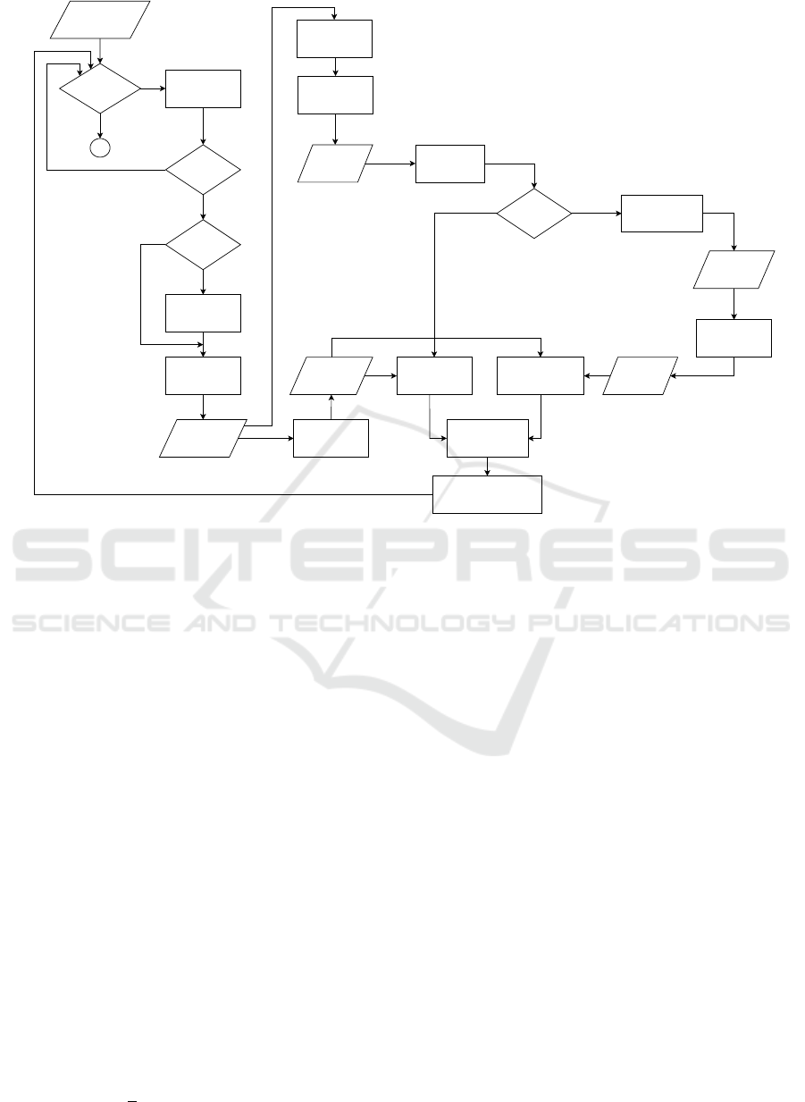
ment classification. Figure 1 shows an overview of
the system containing these components. Overall, the
system workflow proceeds as follows.
1. Video is captured at 30 ms intervals. This is
appropriate because humans typically speak only
one phoneme during a 30 ms interval. We detect
and track the face in the video. Each face image is
cropped to have a width of 800 pixels and a height
of 450 pixels and is then resized to 96 ×96 (cf.
Subsection 2.1);
2. After that, we detect mouth landmarks and resize
the detected mouth region to 28 ×28. The mouth
is classified as to whether it is either closed or
open using a small CNN (cf. Subsection 2.2);
3. When the mouth is closed, sentiment is predicted
using a small CNN with the face only (cf. Sub-
section 2.3);
4. Otherwise, a spectrogram (of size 400 ×400) is
created from the audio signal and is processed
with the face image concurrently; audio features
and video features are concatenated prior to over-
all classification by another lightweight CNN (cf.
Subsection 2.4).
At test time, predictions for each frame are accumu-
lated according to an exponentially-weighted moving
average to yield the final prediction
a
s
t
←
(
y
s
0
, t = 0
α · ˆy
s
t
+ (1 −α) ·a
s
t−1
, t > 0;
(1)
Here, vector ˆy
s
t
represents the predicted distribution
for time t, vector a
s
t
represents the accumulated pre-
dicted distribution at time period t, and the coefficient
α ∈ (0,1) controls the amount of smoothing, with a
higher α discounting older ˆy
s
t
faster. Finally, the ana-
lyzer outputs the sentiment class with the highest esti-
mated probability. We explain each step of the work-
flow in detail in the following subsections.
2.1 Face and Mouth Detection
As indicated in Figure 1, video frames are extracted
every 30 ms from the input video stream. To deter-
mine if there is a face in the frame, we use the classic
Histogram of Oriented Gradient (HOG) detector with
a linear SVM and tracking as implemented by the
dlib library (Dalal and Triggs, 2005). We further use
dlib’s facial landmark detector to find fiducial points
on the face and mouth. Note that dlib implements the
method of (Kazemi and Sullivan, 2014), which yields
68 landmark points such as the corners of the eyes
and the nasal tip. The 68 points are computed rela-
tive to the mean of all the coordinates throughout the
face image. Once the face and its mouth region are de-
tected in a frame, we extract crops as separate images.
The mouth is delineated by dlib landmarks numbered
49 – 63. Each face is resized to 450 ×800. These
images are subsequently used by our mouth classifier,
visual sentiment analysis model, and audiovisual sen-
timent analysis model.
2.2 Mouth Classification
To determine whether a mouth is open or closed, we
use a small CNN consisting of five layers. We resize
Multimodal Sentiment Analysis on Video Streams using Lightweight Deep Neural Networks
443
Video stream
at 30 ms / frame
Detect and track
human face
Face present ?
First face found?
Reinitialize
queue
Crop and resize
to 450 x 800
450 x 800
3-channel
image
Mouth detection
Crop and resize
mouth region
to 28 x 28
Resize to 96 x 96
Visual sentiment
analysis model
(Figure 3)
Audiovisual sentiment
analysis model
(Figure 4)
Accumulate
weighted average
Spectrogram
Convert to
spectrogram
Audio samples
(30ms)
Is mouth open?
YesNo
End of stream?
No
Yes
No
Yes
No
Mouth image
Mouth motion
classification
(Figure2)
End
Start buffering audio
data at 48 kHz.
Yes
96 x 96
3-channel
image
Sentiment prediction
(negative, neutral, positive)
Figure 1: Overall system diagram of the proposed approach.
the input mouth image to a fixed size of 28 ×28 ×3.
The CNN uses two convolutional layers with ReLU
activation and max-pooling followed by two fully-
connected layers, also with ReLU activations, fol-
lowed by a logistic sigmoid classifier. The output rep-
resents the posterior probability that the input repre-
sents an “open” mouth, which we threshold at 0.5 to
obtain the prediction from the network
a
m
t
← ˆy
m
t
≥ 0.5, (2)
where ˆy
m
t
represents the posterior probability output
by the logistic classifier at time t and a
m
t
represents
the predicted mouth state at time t. Figure 2 and Ta-
ble 1 show the model architecture and parameters, re-
spectively. All weights are initialized using Xavier’s
method (Glorot and Bengio, 2010).
2.3 Visual Sentiment Analysis
When the mouth in a frame is closed, the speaker’s
sentiment is analyzed solely from the facial expres-
sion in that frame using the small CNN described in
Figure 3 and Table 2, with an input image size of
96 ×96, a softmax output, and the cross entropy loss
−
1
n
n
∑
i=1
3
∑
k=1
y
(i)
k
log( ˆy
(i)
k
), (3)
where n denotes the batch size, y
(i)
k
is the target (0
or 1) for class k for the i-th instance, and ˆy
(i)
k
is the
predicted probability that the i-th instance belongs to
class k. The model outputs a probability distribution
over the three sentiment classes: positive, negative,
and neutral. Output prediction ˆy
s
t
= [ ˆy
1
, ˆy
2
, ˆy
3
]
>
at
time t is then fed to Equation 1 to obtain an aggre-
gated prediction for the video stream up to time t.
2.4 AudioVisual Sentiment Analysis
When the mouth in a frame is open, the speaker’s
sentiment is analyzed based on both the facial ex-
pression and speech signal in that frame concurrently.
These two types of input are processed by two dif-
ferent small CNNs, which have different-but-similar
structures, as shown in Table 2 (with Figure 3) and
Table 3 (with Figure 4). At a high level, they ex-
ploit the same structure but differ in the dimensions
of each layer due to the different sizes of their in-
put. Moreover, the visual CNN includes dropout to
improve generalization, whereas the audio CNN does
not. The input to the visual CNN is executed in par-
allel with the input to the audio CNN; all layers are
used with ReLU activations. The outputs of the two
modules are concatenated and then piped to a soft-
ICPRAM 2021 - 10th International Conference on Pattern Recognition Applications and Methods
444
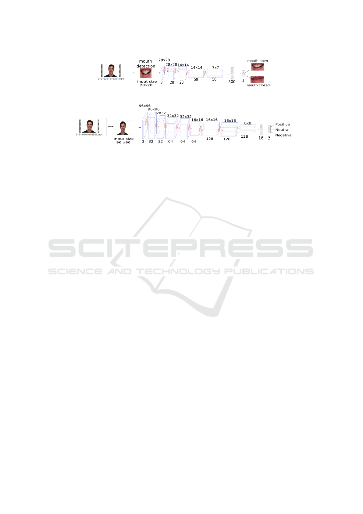
Figure 2: CNN for mouth open / closed classification.
Figure 3: Face-only sentiment classifier.
max layer in order to calculate a probability distribu-
tion over the three sentiment classes. This combined
model is used with RGB images of size 96 ×96 for
the visual input (face) and images of size 400 ×400
for the audio input (spectrogram).
It is worth noting that this module treats the au-
dio signal in the same fashion as an image. A spec-
trogram is a two-dimensional representation of fre-
quency spectra, with time along the horizontal axis
and frequency along the vertical axis. We generate
spectrograms for the audio signal in real time along
with the video frames then pass them to the audio
CNN in the same way ordinary images are fed to an
image CNN. We use a short time Fourier transform
(STFT) to compute the complex-valued spectrogram
S
c
(n,k), where n and k are the time frame and fre-
quency indices, respectively:
S
c
(n,k) ←
W
2
−1
∑
l=−
W
2
w(l) ·x(l + nh) ·e
−2πilk/W
(4)
To compute the STFT, the audio signal x(n) is sliced
into overlapping segments of length W . Each segment
is offset in time by a hop size h. Each segment is
multiplied element-wise by a Hanning window w(l)
that acts as a tapering function to reduce spectral leak-
age. Finally, a DFT of size W is computed separately
on each windowed waveform segment to generate the
spectrogram (Lyon, 2009). Each pixel in the spectro-
gram image represents the magnitude of the complex
value S
c
(n,k) in decibels. Note that, for any com-
plex number z, the magnitude can be calculated by
|z| =
√
a
2
+ b
2
where a and b represent the real and
imaginary parts, respectively.
Like the visual analyzer, the combined model is
trained to minimize the cross-entropy loss (Equation
3). The output predictions ˆy
s
t
at time t are further ac-
cumulated using Equation 1 to yield a final prediction
for the video stream. Overall, the proposed model has
2,646,107 parameters (cf. Tables 1 – 4).
3 EXPERIMENTS
In this section, we specify the dataset used to eval-
uate the system and demonstrate the effectiveness of
the proposed method for sentiment analysis on video
streams. We use Keras version 2.3.1 with TensorFlow
version 2.2.4 as its backend, with OpenCV version 4.2
for all experiments.
3.1 Dataset
We use the Ryerson audio-video database of emo-
tional speech (RAVDESS) (Livingstone and Russo,
2018). RAVDESS is an audio and visual database
of emotional speech and song. The dataset was col-
lected from 24 professional actors and includes eight
emotion categories: neutral, calm, happy, sad, angry,
fearful, disgusted, and surprised. All sequences in the
dataset are available in face-and-voice, face-only, and
voice-only formats. However, we only use the audio-
video format.
Since our system comprises four subsystems for
face-mouth detection, mouth classification, visual
sentiment classification, and audiovisual sentiment
classification (cf. Section 2), we created training
datasets for each module separately. We generated
separate sets of mouth images, face images, audio
files, and corresponding spectrogram images as the
training dataset. We explain the generation steps in
detail here. First, to create the mouth dataset, we used
six actors from RAVDESS and an additional video
from a webcam for one person. For each sequence,
we ran the dlib landmark detector, extracted the
mouth region, randomly sampled 832 mouth regions,
and manually classified each sample mouth as open
or closed. Second, to create the face dataset, we
manually classified face images for 19 actors into
five categories: neutral, calm, happy, angry, and sad
(leaving out surprised and fearful sequences, as they
Multimodal Sentiment Analysis on Video Streams using Lightweight Deep Neural Networks
445

Table 1: Mouth classifier.
Index Layer Kernel Filter
Stride /
Padding
Activation Parameters Input Output
1 input 2,352 0 28 ×28 ×3 28 ×28 ×3
2 convolution1 + ReLU 5 ×5 20 1 / 2 15,680 1,520 28 ×28 ×3 28 ×28 ×20
3 max pooling + dropout (25%) 2 ×2 20 2 / 0 3,920 0 28 ×28 ×20 14 ×14 ×20
4 convolution2 + ReLU 5 ×5 50 1 / 2 9,800 25,050 14 ×14 ×20 14 ×14 ×50
5 max pooling + dropout (25%) 2 ×2 50 2 / 0 2,450 0 14 ×14 ×50 7 ×7 ×50
6 fully connected layer + ReLU 500 1,225,500 2,450 ×1 500 ×1
7 logistic classifier 1 501 500 ×1 1 ×1
Total 1,252,571
Table 2: Visual CNN.
Index Layer Kernel Filter
Stride /
Padding
Activation Parameters Input Output
1 input 27,648 0 96 ×96 ×3 96 ×96 ×3
2 convolution1 + ReLU 3 ×3 16 1 / 1 147,456 448 96 ×96 ×3 96 ×96 ×16
3 batch normalization 147,456 64 96 ×96 ×16 96 ×96 ×16
4 max pooling + dropout (25%) 3 ×3 16 3 / 0 16,384 0 96 ×96 ×16 32 ×32 ×16
5 convolution2 + ReLU 3 ×3 32 1 / 1 32,768 4,640 32 ×32 ×16 32 ×32 ×32
6 batch normalization 32,768 128 32 ×32 ×32 32 ×32 ×32
7 convolution3 + ReLU 3 ×3 32 1 / 1 32,768 9,248 32 ×32 ×32 32 ×32 ×32
8 batch normalization 32,768 128 32 ×32 ×32 32 ×32 ×32
9 max pooling + dropout (25%) 2 ×2 32 2 / 0 8,192 0 32 ×32 ×32 16 ×16 ×32
10 convolution4 + ReLU 3 ×3 64 1 / 1 16,384 18,496 16 ×16 ×32 16 ×16 ×64
11 batch normalization 16,384 256 16 ×16 ×64 16 ×16 ×64
12 convolution5 + ReLU 3 ×3 64 1 / 1 16,384 36,928 16 ×16 ×64 16 ×16 ×64
13 batch normalization 16,384 256 16 ×16 ×64 16 ×16 ×64
14 max pooling + dropout (25%) 2 ×2 64 2 / 0 4,096 0 16 ×16 ×64 8 ×8 ×64
15 fully connected layer + ReLU 16 65,552 4,096 ×1 16 ×1
16 batch normalization 16 64 16 ×1 16 ×1
17 softmax classifier 3 51 16 ×1 3 ×1
Total 136,259
Table 3: Audio CNN.
Index Layer Kernel Filter
Stride /
Padding
Activation Parameters Input Output
1 input 480,000 0 400 ×400 ×3 400 ×400 ×3
2 convolution1 + ReLU 3 ×3 32 1 / 1 5,120,000 896 400 ×400 ×3 400×400 ×32
3 batch normalization 5,120,000 128 400 ×400 ×32 400 ×400 ×32
4 max pooling 3 ×3 32 3 / 0 566,048 0 400 ×400 ×32 133 ×133 ×32
5 convolution2 + ReLU 3 ×3 64 1 / 1 1,132,096 18,496 133 ×133 ×32 133 ×133 ×64
6 batch normalization 1,132,096 256 133 ×133 ×64 133 ×133 ×64
7 convolution3 + ReLU 3 ×3 64 1 / 1 1,132,096 36,928 133 ×133 ×64 133 ×133 ×64
8 batch normalization 1,132,096 256 133 ×133 ×64 133 ×133 ×64
9 max pooling 2 ×2 64 2 / 0 278,784 0 133 ×133 ×64 66 ×66 ×64
10 convolution4 + ReLU 3 ×3 128 1 / 1 557,568 73,856 66 ×66 ×64 66 ×66 ×128
11 batch normalization 557,568 512 66 ×66 ×128 66 ×66 ×128
12 convolution5 + ReLU 3 ×3 128 1 / 1 557,568 147,584 66 ×66 ×128 66 ×66 ×128
13 batch normalization 557,568 512 66 ×66 ×128 66 ×66 ×128
14 max pooling 2 ×2 128 2 / 0 139,392 0 66 ×66 ×128 33 ×33 ×128
15 fully connected layer + ReLU 16 2,230,288 139,392 ×1 16 ×1
16 batch normalization 16 64 16 ×1 16 ×1
17 softmax classifier 3 51 16 ×1 3 ×1
Total 2,509,827
do not express clear sentiment typical of everyday
human interaction), then randomly sampled 1,200
positive, negative, and neutral faces from these sets.
Finally, we prepared the audio data. To be consistent
with the face and mouth image data, we segmented
the RAVDESS audio into chunks 30 ms long using
ICPRAM 2021 - 10th International Conference on Pattern Recognition Applications and Methods
446
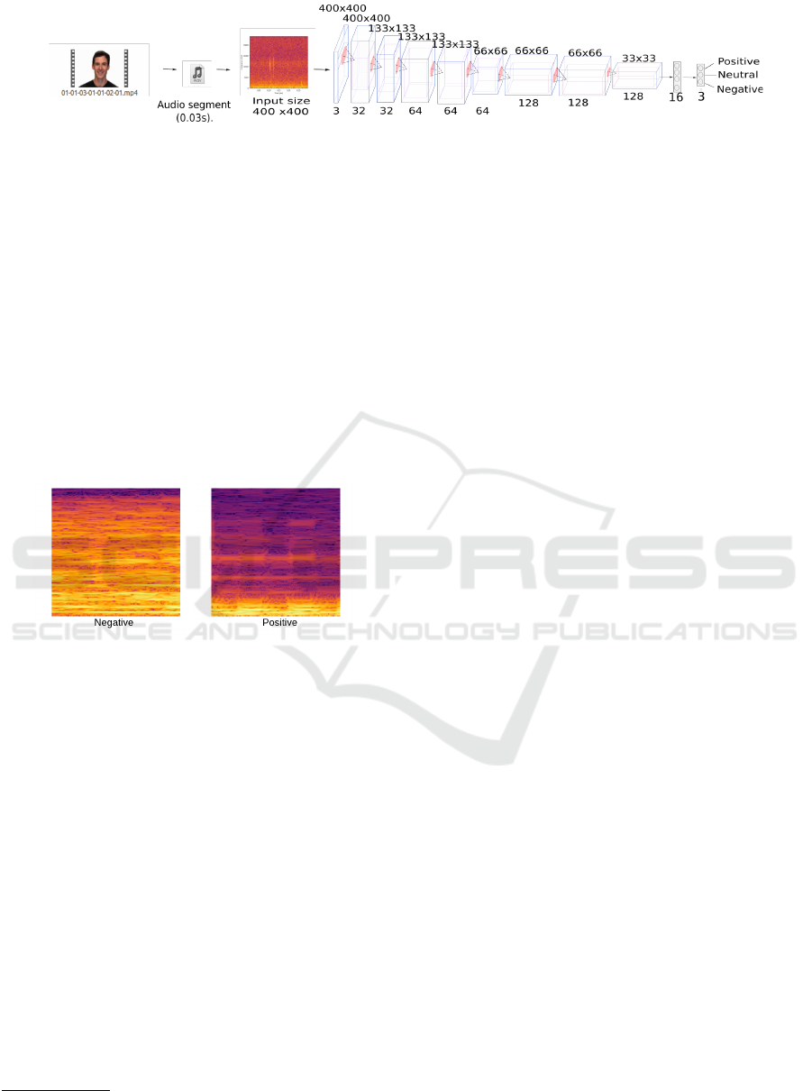
Figure 4: Spectrogram-only sentiment classifier.
pydub.
1
We applied the STFT using scipy
2
to acquire
spectrogram images as frequency-domain representa-
tions of the original signals. We set a sampling rate
of 48 kilohertz, a window size W of 1,400, and 250
overlapping samples between neighboring segments.
All spectrogram elements were converted to a deci-
bel scale. Figure 5 shows spectrogram examples for a
positive sentiment sample (right) and a negative senti-
ment sample (left). The x-axis represents time (in sec-
onds), and the y-axis represents frequency (in Hertz).
The brightness of each pixel indicates the log magni-
tude for a frequency over the window at a particular
time. The x-axis range is 0 – 0.03 seconds, and the
y-axis range is 0 – 24 kHz.
Figure 5: Sample spectrograms for negative (left) and posi-
tive (right) audio.
The test data are organized into three categories:
mouth images (open mouth and closed mouth), sam-
pled video streams for RAVDESS, and sampled video
streams from a web camera. First, we cropped the
mouth region for five RAVDESS actors that were not
used for training. The mouth test set has 200 mouth
images (open mouth and closed mouth). Second, we
used 54 RAVDESS video files from six actors (both
males and females) to test the audio sentiment model,
the visual sentiment model, and the audiovisual senti-
ment model. We also randomly selected video of the
six actors (as our in-sample dataset), balanced so that
each actor provides 9 videos consisting of three pos-
itive, three neutral, and three negative videos. Third,
we used 9 sampled video streams from web camera
videos of three actors (as our out-of-sample dataset),
providing an additional three positive, three neutral,
and three negative videos. These video streams’
1
http://pydub.com/
2
https://docs.scipy.org/doc/scipy/reference/signal.html
lengths range from 4 – 5 seconds. Tables 5 and 6
summarize the size of each dataset constructed as de-
scribed above. We explain how the datasets were used
for training and testing in the next subsection.
3.2 Experimental Setting and
Evaluation Results
We set up each deep learning model as described in
Section 2. We retained 25% of the training data for
validation. The training parameters were as follows.
For the visual CNN, we used the Adam opti-
mizer (Kingma and Ba, 2014) with a batch size of
32 samples, a learning rate of 0.001, a decay of
0.00002, and otherwise the default hyper-parameters
suggested by the authors. The network was trained
for 50 epochs. We compared results with and with-
out augmenting the dataset by up to 25 degrees in
rotation, 0.1 for width shift, 0.1 for height shift, 0.2
for shear range, 0.2 for zoom-in, a horizontal flip,
all using the nearest fill mode. Table 7 shows that
training accuracy and training loss with augmenta-
tion are 91.25% and 0.2185, respectively, compared
to 99.31% and 0.0186, respectively, without augmen-
tation. Hence, we used no augmentation for the visual
image classifier when testing. For the audio CNN,
we again used the Adam optimizer with the same set-
tings as the visual CNN, but with no augmentation,
given that the images are spectrograms for while aug-
mentation would introduce uncertain about frequency.
The network was likewise trained for 50 epochs. Ta-
ble 7 shows that the training accuracy and training
loss with augmentation are 61.18% and 0.813, respec-
tively, compared to 100% and 0.0022, respectively,
without augmentation. Hence, we also used no aug-
mentation for the audio classifier when testing.
For the audiovisual CNN, we first trained the
mouth model with mouth samples partitioned as
shown in Table 5. The training parameters of the
mouth classifier were as follows: Adam optimization
with a batch size of 32 samples and the same hyper-
parameters setting as above, except that mouth data
augmentation used a 30 degrees rotation range. We
trained the mouth CNN for 50 epochs. The resulting
training accuracy, validation accuracy, and test accu-
racy are 99.34%, 99.46% and 97.00% as shown in Ta-
Multimodal Sentiment Analysis on Video Streams using Lightweight Deep Neural Networks
447
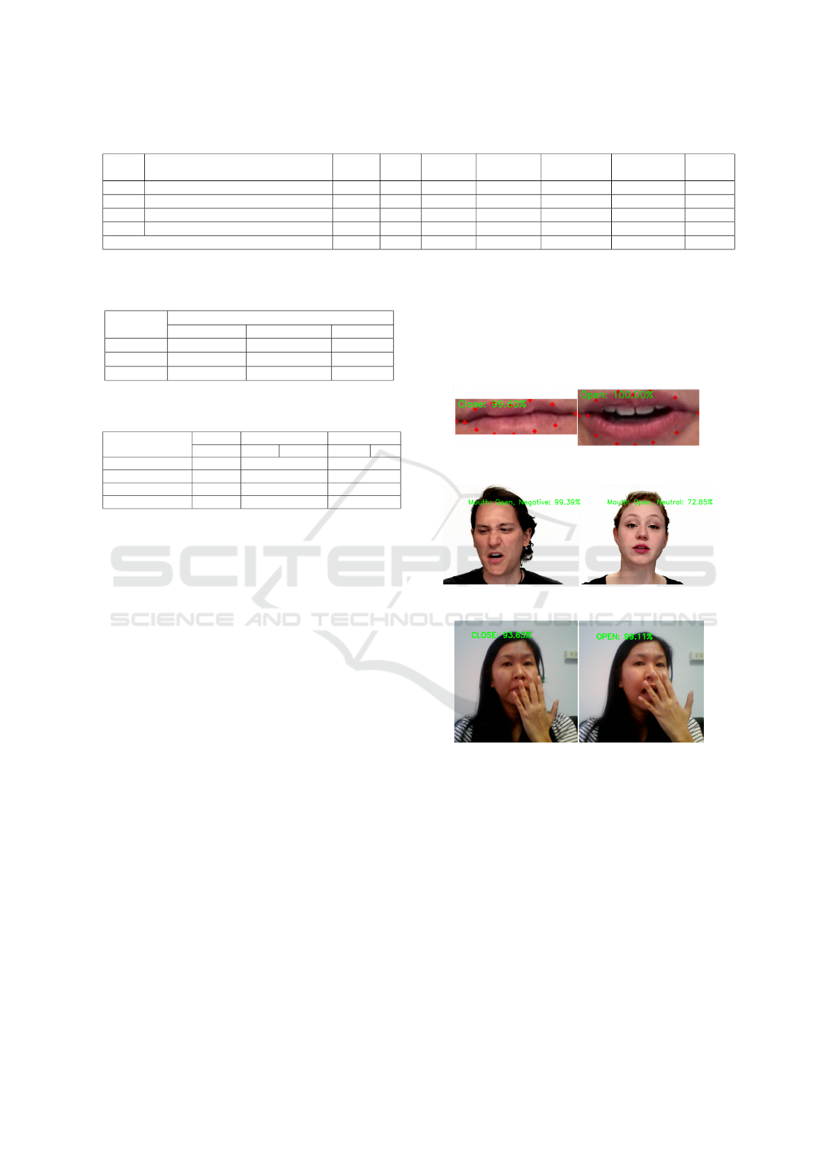
Table 4: AudioVisual CNN.
Index Layer Kernel Filter
Stride /
Padding
Activation Parameters Input Output
1 input from layer 17 of face classifier 3 51 16 ×1 3 ×1
2 input from layer 17 of audio classifier 3 51 16 ×1 3 ×1
3 concatenation 6 0 3 ×1 + 3 ×1 6 ×1
4 softmax classifier 3 21 6 ×1 3 ×1
Total 2,646,107
Table 5: Number of mouth sample images for each senti-
ment class in training, validation, and test sets.
Dataset
Mouth motion
Mouth Open Mouth Closed Accuracy
Training 666 666 99.34%
Validation 166 166 99.46%
Test 200 200 97%
Table 6: Number of spectrogram and face images for each
sentiment class in training, validation, and test sets.
Dataset
Positive Neutral Negative
Happy Calm Neutral Angry Sad
Training 960 960 960
Validation 240 240 240
Test (RAVDESS) 18 files 18 files 18 files
Test (vid. stream) 3 files 3 files 3 files
ble 5. Finally, the mouth CNN was used to determine
which CNN model the input frame should be classi-
fied by. We concatenated the trained CNN models as
explained in Subsection 2.4. The parameters of the in-
tegrated model were learned with stochastic gradient
descent, a batch size of 32 samples, and a learning rate
of 0.01 without weight decay. We trained this model
for 50 epochs and achieved 99.89% training accuracy
(cf. Table 7). Table 8 shows a confusion matrix for
the audiovisual CNN on the validation subset.
To investigate the effectiveness of the proposed
system in a final test, we used both the visual-
only sentiment classifier and the audio-only senti-
ment classifier as baseline models. We computed
the number of correct predictions from the in-sample
test dataset (RAVDESS) and the out-of-sample test
dataset (webcam streams) for our fusion model and
the baselines. A prediction was made for each video
using Equation 1 with y
s
0
= 0 and α = 0.1. Using
audiovisual sentiment feature fusion, we achieved a
90.74% accuracy for the in-sample test dataset and
66.67% accuracy for the out-of-sample test dataset.
This shows that our system can perform better than
the baselines of 11.11% – 31.48% on a challenging
dataset. Indeed, using either single modality yielded
lower test accuracy on both datasets. Sample real-
time system outputs are shown in Figures 6 and 7. The
experimental results are presented in Tables 9 and 10.
As for special conditions, we performed addi-
tional tests of the system’s tolerance to partial occlu-
sion and rotation on the roll axis. We found that if the
subject’s hand is only partially covering the mouth,
dlib will generally find the visible landmarks on the
rest of the mouth. Thus, the audiovisual sentiment
feature classification can proceed. Sample real-time
system outputs for such cases are shown in Figure 8.
Figure 6: Real-time output of mouth motion.
Figure 7: Real-time output of sentiment analysis.
Figure 8: Real-time mouth classification under partial oc-
clusion is generally successful.
4 COMPARISON WITH THE
STATE OF THE ART
(He et al., 2019) propose a preprocessing tech-
nique followed by emotion classification using faces
only. The preprocessing technique comprises three
steps: face detection, face alignment, and frame
subtraction. Frame subtraction is used to capture
changes in expression between subsequent frames.
The authors experiment with GoogleNet, ResNet, and
AlexNet, achieving accuracies of 62.89%, 75.89%,
and 79.74%, respectively. Though the AlexNet-based
ICPRAM 2021 - 10th International Conference on Pattern Recognition Applications and Methods
448

Table 7: Model training results.
Epoch 50
Model
Audio Visual Visual with Augmentation AudioVisual
Images size 400 ×400 96 ×96 96 ×96 400 ×400 + 96 ×96
Training accuracy 100% 99.31% 91.25% 99.89%
Training loss 0.0022 0.0186 0.2185 0.0162
Validation accuracy 53.89% 99.58% 97.36% 88.78%
Validation loss 1.7694 0.0164 0.1090 0.3083
Table 8: Validation confusion matrix.
Actual
Sentiment
Predicted Sentiment
Negative Neutral Positive
Negative 0.72 0.006 0.26
Neutral 0.03 0.84 0.121
Positive 0.07 0.06 0.85
Table 9: Accuracy of in-sample test set prediction.
RAVDESS 6 Actors
(Male and Female)
Video.mp4
Amount
Amount of Correct
Prediction from Model
Visual Audio AudioVisual
1. Positive 18 Files 11 0 13
2. Neutral 18 Files 16 16 18
3. Negative 18 Files 16 16 18
Accuracy 79.63% 59.26% 90.74%
Table 10: Accuracy of out-of-sample test set prediction.
Video Stream
3 Actors
Video Stream
Amount
Amount of Correct
Prediction from Model
Visual Audio AudioVisual
1. Positive 3 Files 3 0 3
2. Neutral 3 Files 0 0 0
3. Negative 3 Files 2 3 3
Accuracy 55.56% 33.33% 66.67%
approach has a similar accuracy to our visual CNN,
our audiovisual CNN performs much better and is
much smaller than AlexNet (61M parameters).
(Rzayeva and Alasgarov, 2019) also attempt emo-
tion recognition from RAVDESS using faces only.
They develop five CNN-based models, among the top
performer is inspired by VGG16. The model uses in-
put images of size 128 ×128. Frames are extracted
every 0.5 seconds and are preprocessed by convert-
ing to grayscale, cropping, and scaling. The model
has 300K parameters and achieves 92% training ac-
curacy, which is less accurate than the training accu-
racy of our visual CNN (cf. Table 7). However, the
authors do not discuss their test performance or how
the approach should be used for real-time sentiment
classification for video streams.
Regarding emotion recognition with RAVDESS
from audio signals only, (Rajak and Mall, 2019)
develop two different CNNs based on 1D and 3D
convolutions. In their experiments, RAVDESS au-
dio is sampled at 44.1 kHz, and Mel-frequency cep-
stral coefficients (MFCCs) are extracted as features.
Their 1D CNN predicts emotion from the waveform,
whereas their 3D CNN classifies according to valence
and arousal. The 1D CNN achieves 49.5% accuracy
on emotion prediction, whereas the 3D CNN achieves
76.2% accuracy on the valence-arousal quadrant pre-
diction task.
For audiovisual emotion recognition, (Jannat
et al., 2018) fuse features learned from both video and
audio, with face image detection and cropping; also,
audio signals are converted into 2D waveform images.
Faces are taken from BP4D+ (Zhang et al., 2016), and
audio signals are taken from RAVDESS. The audiovi-
sual inputs are concatenated then input to Inception-
v3 (a model with 23.83M parameters). The authors
conduct experiments based on image only, audio only,
and both image and audio, achieving training accu-
racy of 99.22%, 66.41%, and 96.09%, respectively.
These four systems use the same RAVDESS test set
that we do. However, our training and test data are
different random samples from the larger dataset, so
we may expect some small deviation due to sampling.
Nevertheless, we demonstrate higher accuracy than
the existing work on the training data (0.09% better
for visual, 33.59% better for audio, and 3.8% better
for audiovisual). Also, while (Jannat et al., 2018) do
not report test accuracy at all, we obtain high accuracy
for the in-sample test set and acceptable accuracy for
the out-of-sample test set (cf. Tables 9 and 10). Our
model size is also much smaller, meaning it can be
used in a resource-constrained environment. Finally,
our deep fusion system also accounts for dynamic
emotion in video streams by predicting per frame and
also accumulating information over multiple frames
prior to making a prediction.
5 DISCUSSION AND FUTURE
DIRECTIONS
This paper introduces a method for deep audiovisual
multimodal sentiment analysis on video streams by
synthesizing small neural networks to deal with open
and closed mouths differently. We conduct compre-
hensive experiments with a RAVDESS test set and
an out-of-sample test dataset to show that emotional
expressions of a subject can be estimated accurately
with the use of multiple modalities. We achieve
Multimodal Sentiment Analysis on Video Streams using Lightweight Deep Neural Networks
449

90.74% in-sample test accuracy using the proposed
system. The experiments also show that using both
visual and audio features improves performance. Our
model is very good at predicting negative and neutral
sentiment, but it is less effective at predicting pos-
itive sentiment. We hypothesize that the lower ac-
curacy for positive sentiment is due to a low num-
ber of happy video samples in RAVDESS. Moreover,
in the positive samples, positive sentiment is not ex-
pressed in every frame. In frames of the positive-
labeled videos, the subjects actually evince a neu-
tral sentiment. Thus, at test time, the model may
over-estimate the probability of neutral sentiment in
the happy sample. As a final observation, test accu-
racy with the out-of-sample dataset is lower than with
the in-sample dataset. We suppose this is because
the RAVDESS actors are Caucasian Americans, while
our out-of-sample actors are Asian.
It is worth mentioning again that we target real-
time sentiment monitoring for retail businesses; hence
the size of the neural networks used in the system
is very important, and our work compares favorably
with larger state-of-the-art models such as Inception-
ResNet-v2 and VGG16 in size. In the future, we
will employ our solution at commercial scale, e.g, to
predict customer satisfaction in multiple SME retail
shops, which usually have limited willingness to in-
vest in software and hardware capability. Moreover,
we will improve the out-of-sample performance of
our system and explore alternative methods to accu-
mulate information over a period of time.
REFERENCES
Avots, E., Sapi
´
nski, T., Bachmann, M., and Kami
´
nska, D.
(2019). Audiovisual emotion recognition in wild. Ma-
chine Vision and Applications, 30(5):975–985.
Cambria, E., Schuller, B., Xia, Y., and Havasi, C. (2013).
New avenues in opinion mining and sentiment analy-
sis. IEEE Intelligent systems, 28(2):15–21.
Chen, M., Yang, J., Zhu, X., Wang, X., Liu, M., and Song, J.
(2017). Smart home 2.0: Innovative smart home sys-
tem powered by botanical iot and emotion detection.
Mobile Networks and Applications, 22(6):1159–1169.
Chen, M., Zhang, Y., Qiu, M., Guizani, N., and Hao, Y.
(2018). Spha: Smart personal health advisor based
on deep analytics. IEEE Communications Magazine,
56(3):164–169.
Dalal, N. and Triggs, B. (2005). Histograms of oriented
gradients for human detection. In 2005 IEEE com-
puter society conference on computer vision and pat-
tern recognition (CVPR’05), volume 1, pages 886–
893. IEEE.
Glorot, X. and Bengio, Y. (2010). Understanding the diffi-
culty of training deep feedforward neural networks.
In Proceedings of the thirteenth international con-
ference on artificial intelligence and statistics, pages
249–256.
Harley, J. M., Lajoie, S. P., Frasson, C., and Hall, N. C.
(2015). An integrated emotion-aware framework for
intelligent tutoring systems. In Conati, C., Heffernan,
N., Mitrovic, A., and Verdejo, M. F., editors, Artifi-
cial Intelligence in Education, pages 616–619, Cham.
Springer International Publishing.
He, Z., Jin, T., Basu, A., Soraghan, J., Di Caterina, G., and
Petropoulakis, L. (2019). Human emotion recognition
in video using subtraction pre-processing. In Proceed-
ings of the 2019 11th International Conference on Ma-
chine Learning and Computing, pages 374–379.
Hossain, M. S. and Muhammad, G. (2019). Emotion
recognition using deep learning approach from audio–
visual emotional big data. Information Fusion, 49:69–
78.
Huang, X., Kortelainen, J., Zhao, G., Li, X., Moilanen,
A., Sepp
¨
anen, T., and Pietik
¨
ainen, M. (2016). Multi-
modal emotion analysis from facial expressions and
electroencephalogram. Computer Vision and Image
Understanding, 147:114 – 124. Spontaneous Facial
Behaviour Analysis.
Jannat, R., Tynes, I., Lime, L. L., Adorno, J., and Cana-
van, S. (2018). Ubiquitous emotion recognition us-
ing audio and video data. In Proceedings of the 2018
ACM International Joint Conference and 2018 In-
ternational Symposium on Pervasive and Ubiquitous
Computing and Wearable Computers, pages 956–959.
Kazemi, V. and Sullivan, J. (2014). One millisecond face
alignment with an ensemble of regression trees. In
Proceedings of the IEEE conference on computer vi-
sion and pattern recognition, pages 1867–1874.
Kingma, D. P. and Ba, J. (2014). Adam: A
method for stochastic optimization. arXiv preprint
arXiv:1412.6980.
Lippi, M. and Torroni, P. (2015). Argument mining: A ma-
chine learning perspective. In International Workshop
on Theory and Applications of Formal Argumentation,
pages 163–176. Springer.
Livingstone, S. R. and Russo, F. A. (2018). The ryerson
audio-visual database of emotional speech and song
(ravdess): A dynamic, multimodal set of facial and
vocal expressions in north american english. PloS one,
13(5):e0196391.
Lyon, D. A. (2009). The discrete fourier transform, part 4:
spectral leakage. Journal of object technology, 8(7).
Rajak, R. and Mall, R. (2019). Emotion recognition from
audio, dimensional and discrete categorization using
cnns. In TENCON 2019-2019 IEEE Region 10 Con-
ference (TENCON), pages 301–305. IEEE.
Rzayeva, Z. and Alasgarov, E. (2019). Facial emotion
recognition using convolutional neural networks. In
2019 IEEE 13th International Conference on Applica-
tion of Information and Communication Technologies
(AICT), pages 1–5.
Valstar, M., Gratch, J., Schuller, B., Ringeval, F., Lalanne,
D., Torres Torres, M., Scherer, S., Stratou, G., Cowie,
R., and Pantic, M. (2016). Avec 2016: Depression,
mood, and emotion recognition workshop and chal-
ICPRAM 2021 - 10th International Conference on Pattern Recognition Applications and Methods
450

lenge. In Proceedings of the 6th international work-
shop on audio/visual emotion challenge, pages 3–10.
Wang, S. and Ji, Q. (2015). Video affective content analy-
sis: a survey of state-of-the-art methods. IEEE Trans-
actions on Affective Computing, 6(4):410–430.
Zhang, Z., Girard, J. M., Wu, Y., Zhang, X., Liu, P., Ciftci,
U., Canavan, S., Reale, M., Horowitz, A., Yang, H.,
Cohn, J. F., Ji, Q., and Yin, L. (2016). Multimodal
spontaneous emotion corpus for human behavior anal-
ysis. In 2016 IEEE Conference on Computer Vision
and Pattern Recognition (CVPR), pages 3438–3446.
Multimodal Sentiment Analysis on Video Streams using Lightweight Deep Neural Networks
451
