On Power Jaccard Losses for Semantic Segmentation

David Duque-Arias

1 a

, Santiago Velasco-Forero

1 b

, Jean-Emmanuel Deschaud

1 c

Franc¸ois Goulette

1 d

, Andres Serna

2 e

, Etienne Decenci

ere

1 f

and Beatriz Marcotegui

1 g

MINES ParisTech, PSL Research University, France

Terra3D Research, Paris, France

Keywords:

Loss Functions, Image Segmentation, Jaccard Loss, Deep Learning, U-Net Architecture.

Abstract:

In this work, a new generalized loss function is proposed called power Jaccard to perform semantic seg-

mentation tasks. It is compared with classical loss functions in different scenarios, including gray level and

color image segmentation, as well as 3D point cloud segmentation. The results show improved performance,

stability and convergence. We made available the code with our proposal with a demonstrative example.

1 INTRODUCTION

Image segmentation using learning-based approaches

is an active research topic. One of the most com-

mon issues in this task is related to highly unbal-

anced datasets. Several strategies have been pro-

posed in order to compensate less populated classes.

They can be mainly clustered in two categories: 1)

Data-level methods, increasing artiﬁcially the number

of training samples via data augmentation through

over-sampling and under-sampling training samples;

2) Algorithm-level methods, without modifying the

training data distribution, the decision process in-

creases the importance of smaller classes (Johnson

and Khoshgoftaar, 2019). In this paper, we focus on

the second approach, by modifying the loss function

to penalize model mistakes similar to focal loss (Lin

et al., 2017).

According to (Jun, 2020), loss functions can be

mainly divided in two groups: 1) Statistical-based

such as Cross-Entropy (CE) and some of its variants

such as Weighted CE (Ronneberger et al., 2015), dis-

tance map penalized (Caliv

a et al., 2019) that com-

putes a mask based on pixels that are close to a given

class, Focal loss and top K-loss (Wu et al., 2016) that

drop pixels when they are too easy to classify, given a

threshold parameter.

https://orcid.org/0000-0002-2966-4922

https://orcid.org/0000-0002-2438-1747

https://orcid.org/0000-0002-6696-9354

https://orcid.org/0000-0003-1527-2650

https://orcid.org/0000-0003-2348-3079

https://orcid.org/0000-0002-1349-8042

https://orcid.org/0000-0002-2825-7292

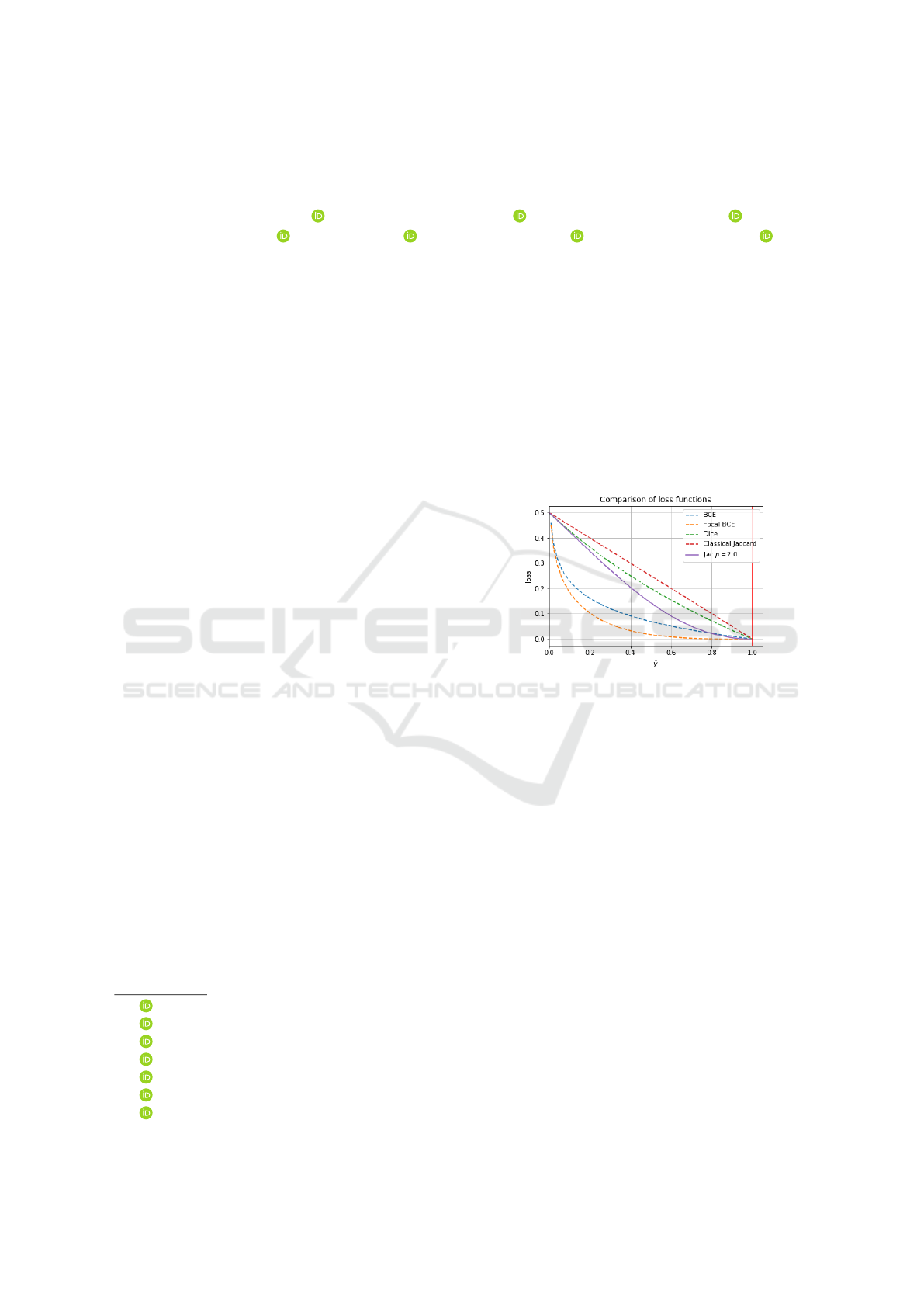
Figure 1: Comparison of some classical loss functions (dot-

ted lines) and our proposed Power Jaccard loss (solid line).

Binary Cross-Entropy. For Focal BCE with γ = 2. Verti-

cal red line indicates the ground truth y = 1. Our proposal

reduces the relative loss for well-classiﬁed examples.

2) Geometrical-based loss functions inspired by

discrete sets and mostly motivated by Sørensen-Dice

score. As an extension of Dice, Tversky loss (Salehi

et al., 2017) allows to penalize differently False Pos-

itives (FP) and False Negatives (FN); well known

Jaccard loss or Intersection over Union (IoU) (Po-

lak et al., 2009) and its multiclass version mean IoU;

boundary loss (Kervadec et al., 2018) takes the form

of a distance metric in the space of contours. Penalty

Generalized Dice (pGD) (Yang et al., 2019) seeks to

penalize with an additional parameter both FP and

FN. Geometrical-based loss functions are an active

research ﬁeld with successful results in semantic seg-

mentation (Sudre et al., 2017).

During 3D point cloud challenge SHREC’20

(Zolanvari et al., 2019), we compared several losses

to improve semantic segmentation (Ku et al., 2020).

We found that some deep learning architectures such

as Unet or SegNet (Badrinarayanan et al., 2017) did

not achieve high performance as expected, using the

Duque-Arias, D., Velasco-Forero, S., Deschaud, J., Goulette, F., Serna, A., Decencière, E. and Marcotegui, B.

On Power Jaccard Losses for Semantic Segmentation.

DOI: 10.5220/0010304005610568

In Proceedings of the 16th International Joint Conference on Computer Vision, Imaging and Computer Graphics Theory and Applications (VISIGRAPP 2021) - Volume 5: VISAPP, pages

561-568

ISBN: 978-989-758-488-6

561

most common loss functions such as Focal loss, clas-

sical cross-entropy and Jaccard loss. Obtained results

motivated us to propose a loss function able to penal-

ize wrong predicted labels and to focus more on them

to improve the general performance.

Our main contribution in this paper is a general-

ization of Jaccard loss function for image segmenta-

tion. In proposed loss, the higher the power term, the

stronger the penalization of the worst predicted sam-

ples. We have evaluated our proposal with several

segmentation datasets such as MNIST, Cityscapes

(Cordts et al., 2016), SHREC’20 point clouds and

aerial images (Mnih, 2013). The use of power losses

improves the performance in binary and multiclass

segmentation (section 4). Fig. 1 illustrates a compar-

ison between the proposed loss functions and other

classical losses as cross-entropy, Jaccard and Dice

score. The abscissas represent the predicted value ˆy

and the ordinates the corresponding loss value. We

will see that a higher value of p in our generalized

Jaccard loss function improves model convergence by

shifting the focus to improve harder predictions.

The structure of the paper is as follows: Section

2 describes the proposed loss function; Section 3 in-

troduces the experimental design to evaluate our pro-

posal; in Section 4 the results of semantic segmenta-

tion comparing several loss functions with different

types of images are reported. Finally, in Section 5 the

conclusions are stated.

2 LOSS FUNCTIONS

In this Section, we present power Jaccard loss gener-

alizing the well known Jaccard index.

2.1 Jaccard Index

The Jaccard index was introduced in (Jaccard, 1901).

It measures the similarity measures the similarity be-

tween ﬁnite sample sets A,B as the Intersection over

Union (IoU):

|A∩B|

|A∪B|

|A∩B|

|A|+|B|−|A∩B|

. The Jaccard in-

dex is zero if the two sets are disjoint and is one if

they are identical. Other similarity index exist such as

Dice’s index deﬁned as

2|A∩B|

|A|+|B|

and it can be rewritten

in terms of Jaccard as

1+J

. For minimization pur-

poses, it is recommended to use the Jaccard distance

= 1 −

|A∩B|

|A∪B|

a.k.a. Steinhaus distance or biotope

distance, which were proposed to compare unordered

sets (Deza and Deza, 2009). During the segmenta-

tion process, the loss function should evaluate each

pixel i measuring the distance between its ground

truth y

∈ {0,1} and the current result of the model ˆy

the estimated probability value representing its like-

lihood of being part of the object. Subscript i is re-

moved for simpliﬁcation reasons in y

and ˆy

. The

straightforward implementation of J

as a loss func-

tion in continuous domain replaces intersection and

union by product and sum as follows ((Rahman and

Wang, 2016) and (Martire et al., 2017)):

(y, ˆy) = 1 −

(y · ˆy) +ε

(y + ˆy −y · ˆy) + ε

(1)

where ε prevents zero division.

(Cha, 2007) uses J

as a variation of the normal-

ized inner product to measure the distance between

density probability functions with a power term equal

to two in the denominator:

(y, ˆy) = 1 −

(y · ˆy) +ε

+ ˆy

− y · ˆy)+ ε

(y − ˆy)

+ ˆy

− y · ˆy)+ ε

(2)

This modiﬁcation from (1) to (2) can be inter-

preted in the context of focal loss, where the main

idea is to reduce both loss and gradient for correct

prediction while emphasizing the gradient of errors

(See Fig. 1).

2.2 Power Jaccard

We propose a generalized loss function called Power

Jaccard Loss including a power term p to the Jaccard

loss of (1) in order to increase the weight of wrong

predictions during training, as follows:

(y, ˆy, p) = 1 −

(y · ˆy) +ε

+ ˆy

− y · ˆy)+ ε

(3)

If p = 1, our proposed loss is identical to Jaccard

distance. Previous works have directly used p = 2 in

geometrical losses such as Dice score (Diakogiannis

et al., 2020) and Jaccard distance (Decenci

ere et al.,

2018).

Fig. 1 illustrates the shape of loss functions ac-

cording to p. We propose to increase the weight of

wrong predicted samples depending on p. Also, as

shows Fig. 2 for p > 2, the minimum of loss function

is not at ˆy = 1. This implies that the model will con-

verge to a non desired optimal value and negative val-

ues of loss would be obtained. We also demonstrate

that p must be between one and two.

3 EXPERIMENTAL DESIGN

Power Jaccard loss is validated in semantic segmen-

tation frameworks with several datasets: MNIST,

VISAPP 2021 - 16th International Conference on Computer Vision Theory and Applications

562

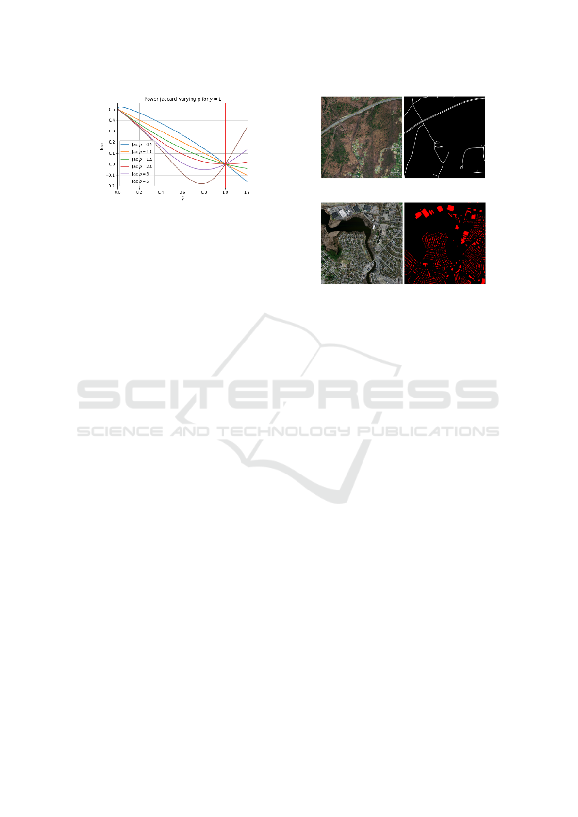
Figure 2: Incidence of parameter p in power Jaccard loss.

Vertical red line indicates the ground truth value of y = 1.

Cityscapes, aerial images from Toronto University

and SHREC’20 challenge. We selected Unet based

architectures and performed some variations to the

model (number of ﬁlters), the training stage (dataset

size and batch size) and compared the incidence of

our proposal. Each conﬁguration is repeated several

times to evaluate stability and repetitiveness, which is

a common issue in neural networks (Scardapane and

Wang, 2017). As evaluation metrics, we used mean

IoU, accuracy and recall scores.

3.1 Grayscale Images

MNIST dataset contains grayscale images of 28x28

pixels with digits of ten classes from zero to nine and

one digit instance by image. We randomly selected

140 images per class and built a pixel-wise ground

truth (Zhou, 2018). Then, the dataset was divided in

the three common subsets as follows: 1000 for train-

ing, 200 for validation and 200 for test.

Two segmentation problems have been tackled:

1) Binary segmentation to distinguish between back-

ground and digit pixels; 2) Multiclass segmentation in

ten classes. In both cases, we selected an Unet model

with three levels of depth where the number of ﬁlters

was changed between two, four and eight. Diverse

batch sizes were used: 1, 10 and 50. Each conﬁgu-

ration was evaluated with different losses: binary or

categorical CE, classical Jaccard and power Jaccard

with several values of p. In all trained models, the in-

put shape is a single channel image. Each experiment

is repeated ﬁve times. The code is available at

3.2 RGB Images

Two color datasets are used: 1) Aerial images

from (Mnih, 2013) for binary segmentation; 2) Urban

The code to train a segmentation model on MNIST

images varying the loss functions is available at:

https://github.com/daduquea/powerLosses/.

(a) Road segmentation.

(b) Building segmentation.

Figure 3: Example of Mnih dataset (RGB and GT).

scenes images from Cityscapes (Cordts et al., 2016)

for multiclass segmentation.

3.2.1 Aerial Images

We performed two binary segmentation tasks: 1)

Road and no-road (1108 images for training, 14 for

validation and 49 for testing); 2) Building and no-

building (137 images for training, four for validation

and ten for testing). Fig. 3 presents two images from

the dataset and the corresponding ground truth.

Unet initialized from ImageNet with Mo-

bileNetV2 (Sandler et al., 2018) as feature extractor

is used. Adam optimizer with a default learning rate

of 10

−3

and a patience equal to ﬁve.

3.2.2 Urban Scene Images

Cityscapes dataset is composed of 5K color images

with divided in three subsets: training (2975), vali-

dation (500) and test (1525) and annotated with 30

classes in the context of autonomous driving. Fig. 4

shows an image from this dataset.

We have selected a subset of four classes relevant

for autonomous driving to perform semantic segmen-

tation in unbalanced data: person, car, road and back-

ground.

3.3 Point Cloud Projections

SHREC’20 dataset contains 80 point clouds, each one

has about three millions points (x,y,z). Each point

cloud of the training set is manually labeled with fol-

lowing classes: building, car, ground, pole and veg-

On Power Jaccard Losses for Semantic Segmentation

563

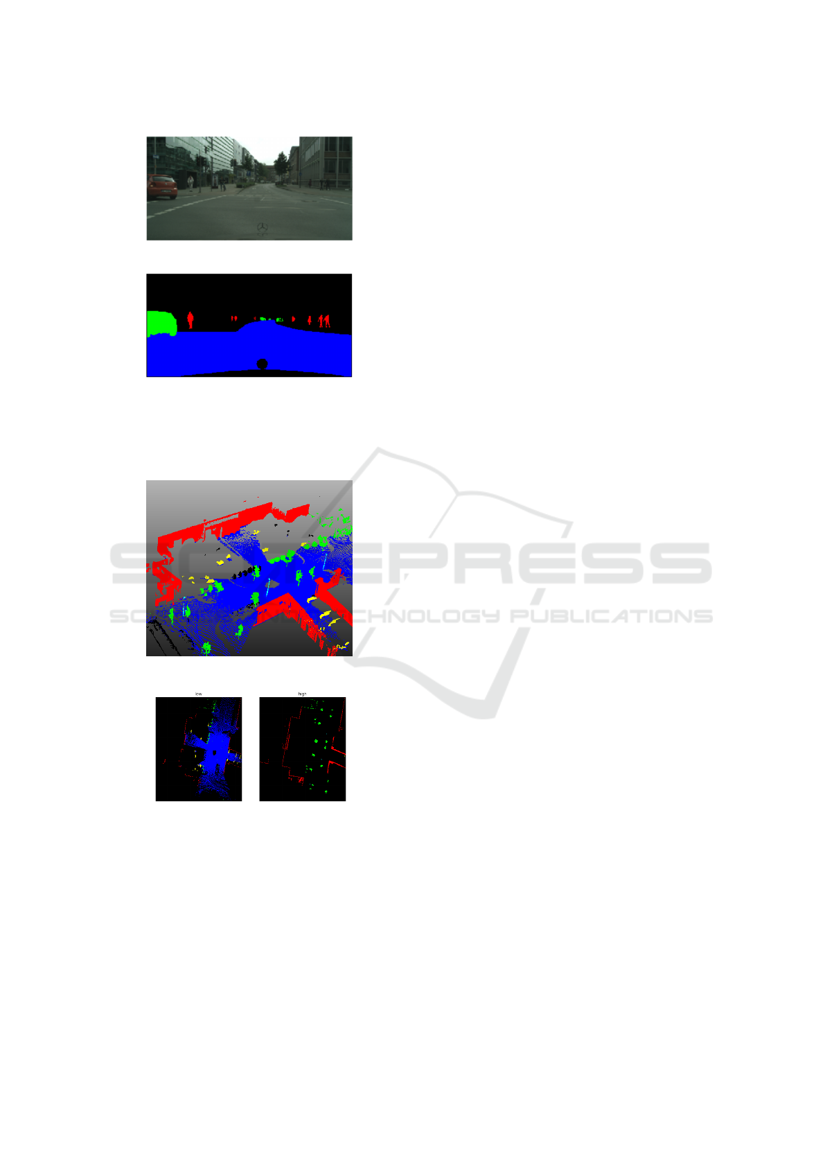
(a) RGB Image.

(b) Ground truth of selected classes.

Color scale for each class: Road is blue,

person is red, car is green and background

is black.

Figure 4: Image from Cityscapes (Cordts et al., 2016).

(a) 3D points.

(b) Bird Eye View (BEV) projections.

Figure 5: Point cloud with ground truth from SHREC’20

challenge (Zolanvari et al., 2019) and the corresponding

BEV projections.

etation. Segmentation is obtained from 2D Bird eye

view (BEV). Fig. 5 shows a point cloud with ground

truth labels.

We divided segmentation of 3D point clouds in

two simpler problems: 1) Segment lower points (low

slice) in building and car classes; 2) Segment higher

points (high slice) in building and vegetation classes.

Fig. 5b shows BEV projections of low and high slice

Fig. 5a.

Ground and poles have been discarded because: 1)

Ground can be extracted using an analytical approach

such as the Lambda Flat Zone method proposed by

(Hern

andez and Marcotegui, 2009) and then extended

for (Serna and Marcotegui, 2014) to compute Digital

Elevation Model (DEM); 2) Pole class is problematic

because a single trafﬁc sign, very different from other

pole instances, contains 70 % of the pole class points

in the whole dataset.

We computed hand crafted features based on the

BEV projections (Serna and Marcotegui, 2014) from

3D point clouds. For the low slice: h

max

and

max(h

max

,∆h

min

) and for the high slice: h

min

, h

max

and ∆h. We note that h

max

and h

min

represent the max-

imum height and the minimum height of all points

that fell in the same pixel, ∆h = h

max

− h

min

and

∆h

min

= h

min

− DEM.

The semantic segmentation task was performed

independently on each slice: one model was trained

in the low slice and another one in the high slice.

Both slices share some common characteristics such

as the same Unet-based architecture with three levels

of depth, the kernel size of convolutions, patience and

Adadelta optimizer with a learning rate of 0.001.

4 RESULTS

In this section we present obtained results in binary

and multiclass segmentation tasks. Power losses out-

performs classical losses in tested scenarios with dif-

ferent kinds of data.

4.1 Gray Scale Images

4.1.1 Binary Segmentation

Experiments with different number of ﬁlters, batch

size and loss functions are performed. Table 1 shows

the results using a batch size equal to one. Mean IoU,

standard deviation and the best IoU of ﬁve runs are

reported.

It was experimentally found that increasing the

batch size negatively affects the performance of the

model. It can be justiﬁed because with a smaller

batch, the model gradually learns to distinguish be-

tween background and a single class. Even though,

over a batch size of 10, the variance of the digit class

increases because it groups a set on non homogeneous

instances of the ten classes. Furthermore, Table 1 re-

ports a high standard deviation for almost all conﬁg-

VISAPP 2021 - 16th International Conference on Computer Vision Theory and Applications

564

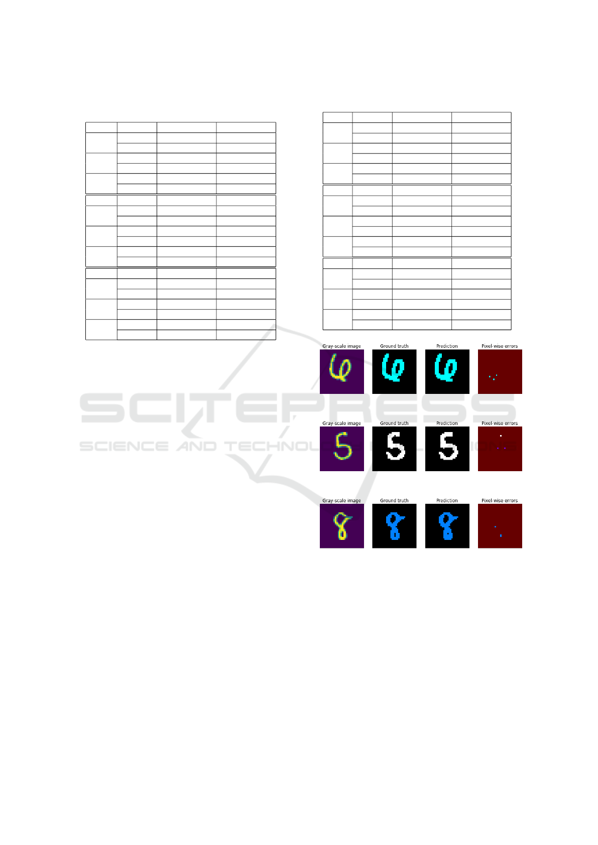
Table 1: Binary segmentation in MNIST dataset with batch

size of one.

Filters Metric CE Jac. p = 1

IoU 0.8542 ± 0.1651 0.4402 ± 0.0298

Best IOU 0.9884 0.5000

IoU 0.8773 ± 0.1889 0.4551 ± 0.0366

Best IOU 0.9878 0.5000

IoU 0.8216 ± 0.1654 0.4403 ± 0.0304

Best IOU 0.9504 0.5011

Filters Metric Jac. p = 1.25 Jac. p = 1.5

IoU 0.5303 ± 0.2101 0.5538 ± 0.2217

Best IOU 0.9507 0.9735

IoU 0.5545 ± 0.2234 0.5396 ± 0.2290

Best IOU 0.9977 0.9566

IoU 0.4348 ± 0.0191 0.5395 ± 0.2290

Best IOU 0.4737 0.9977

Filters Metric Jac. p = 1.75 Jac. p = 2

IoU 0.9813 ± 0.0172 0.7679 ± 0.2797

Best IOU 0.9977 0.9975

IoU 0.6507 ± 0.2760 0.7687 ± 0.2804

Best IOU 0.9938 0.9977

IoU 0.5397 ± 0.2289 0.5397 ± 0.2289

Best IOU 0.9977 0.9977

urations. It implies that during training, models con-

verged to different local minima with different values

at each run.

Power losses allow to train simpler models out-

performing other loss functions. Table 1 shows that

the model with two ﬁlters and power Jaccard with

p = 1.75 obtained a performance equal to the best

model with eight ﬁlters. The improvement obtained

using power losses is higher when training smaller

models. These loss functions could be useful with

low memory requirements.

4.1.2 Multiclass Segmentation

We varied batch size between 1, 10 and 50 and re-

peated ﬁve times each conﬁguration, as presented in

Table 2.

From Table 2, it can be seen that power Jaccard

allows to obtain higher score compared against cross-

entropy and classical Jaccard. Fig. 6 presents some

predictions obtained with the best model achieved us-

ing power Jaccard with p = 2 and batch size of one.

We observed that in the best models, the errors were

in general at pixel-wise level. This type of errors can

be solved by means of regularization techniques such

as voting systems (Alpaydin, 1997).

4.2 RGB Images

4.2.1 Aerial Images

Table 3 presents accuracy values by experiment with

several loss functions. We observe that in both ex-

Table 2: Mean IoU in multiclass segmentation on MNIST.

Batch Metric CE Jac. p = 1

IoU 0.0956 ± 0.0309 0.0000 ± 0.0000

Best IOU 0.1501 0.0000

IoU 0.1341 ± 0.0228 0.4537 ± 0.1014

Best IOU 0.1612 0.6562

IoU 0.1534 ± 0.0101 0.4819 ± 0.0779

Best IOU 0.1679 0.6188

Batch Metric Jac. p = 1.25 Jac. p = 1.5

IoU 0.0062 ± 0.0076 0.4831 ± 0.4031

Best IOU 0.0152 0.9137

IoU 0.5298 ± 0.0963 0.6852 ± 0.0464

Best IOU 0.6378 0.7747

IoU 0.5255 ± 0.1055 0.6364 ± 0.0699

Best IOU 0.7342 0.7432

Batch Metric Jac. p = 1.75 Jac. p = 2

IoU 0.6388 ± 0.3394 0.5160 ± 0.4240

Best IOU 0.8960 0.9450

IoU 0.8307 ± 0.0535 0.7953 ± 0.0499

Best IOU 0.8793 0.8856

IoU 0.7403 ± 0.1137 0.7590 ± 0.0577

Best IOU 0.8342 0.8064

(a) Example 1.

(b) Example 2.

Figure 6: Multiclass segmentation using MNIST dataset.

From left to right: 1) Original gray scale image; 2) Ground

truth generated from gray scale image; 3) Prediction us-

ing best obtained model; 4) Errors between prediction and

ground truth.

periments, the use of power losses leads to better re-

sults by a small margin and highest accuracy was ob-

tained with p = 1.5. One may also note that BCE has

the lowest validation accuracy in both datasets. The

small differences between different loss functions oc-

cur because of to the use of an already trained model

as feature extractor, as described in Section 3.

On Power Jaccard Losses for Semantic Segmentation

565

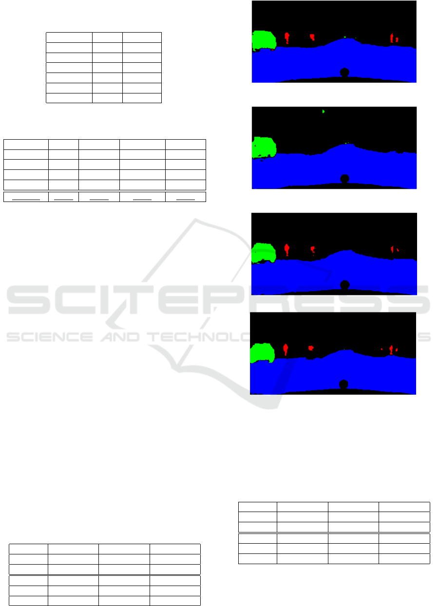
Table 3: Accuracy in validation set on Aerial images. First

column indicates the used loss function: BCE, Focal BCE,

Dice score and power Jaccard.

Roads Buildings

BCE 0.9622 0.9376

F-BCE 0.9677 0.9421

Dice 0.9680 0.9489

Jac. p = 1 0.9676 0.9484

Jac. p = 1.5 0.9684 0.9503

Jac. p = 2 0.9682 0.9502

Table 4: IoU by class and mean IoU in validation set of

Cityscapes (Cordts et al., 2016).

CE Jac. p = 1 Jac. p = 1.5 Jac. p = 2

Person 0.1135 0.0000 0.1118 0.1390

Car 0.4620 0.4004 0.4209 0.5082

Road 0.8380 0.8137 0.8047 0.8263

Background 0.8721 0.8541 0.8605 0.8738

Mean IoU 0.5714 0.5170 0.5495 0.5868

4.2.2 Urban Scene Images

Table 4 reports the results on Cityscapes dataset.

Power losses improve the performance on less pop-

ulated classes such as person and car thanks to the

higher penalty for worst predictions (see Fig. 2).

The relative improvement in IoU between cross-

entropy and power Jaccard with p equal to 2 in back-

ground was 0.1949%, in person was 22.46% and in

car was 10%. On the road, it worsened by 1.39%. In

the mean IoU, the relative improvement was 2.69%.

Fig. 7 shows the predictions of the image presented in

Fig. 4 using the models trained with different losses.

It is seen how the inﬂuence of the power term qualita-

tively improve the segmentation of the person class.

4.3 Point Cloud Projections

This section presents the results of semantic segmen-

tation in 3D point clouds. We divide each point cloud

in two slices: low and high, in order to simplify clas-

siﬁcation problems and focused on the impact of the

loss function. Tables 5 and 6 present obtained results

with several losses. We report three values by loss

function: IoU is the average and the standard devia-

tion of the mean IoU in test set and best IoU is the

highest IoU obtained in test set

Table 5: Performance in low slice from SHREC’20 dataset.

Metric CE Focal BCE Dice score

IoU 0.279 ± 0.426 0.450 ± 0.172 0.665 ± 0.196

Best IOU 0.934 0.797 0.798

Metric Jac. p = 1 Jac. p = 1.5 Jac. p = 2

IoU 0.702 ± 0.230 0.931 ± 0.009 0.925 ± 0.009

Best IOU 0.941 0.943 0.939

(a) Cross-entropy.

(b) Classical Jaccard.

(d) Power Jaccard with p = 2.

Figure 7: Example of Prediction 4 in Cityscapes. Road

(blue), person (red), car (green) and background (black).

Note that Power Jaccard performs better on smaller classes

than the classical one. Quantitative results are given in Ta-

ble 4.

Table 6: Performance in high slice from SHREC’20

dataset.

Metric CE Focal BCE Dice p = 1

IoU 0.341 ± 0.000 0.570 ± 0.016 0.427 ± 0.173

Best IOU 0.341 0.605 0.787

Metric Jac. p = 1 Jac. p = 1.5 Jac. p = 2

IoU 0.341 ± 0.000 0.761 ± 0.144 0.761 ± 0.020

Best IOU 0.341 0.809 0.788

In general, using Power Jaccard, the performance

was better and the models converged more often. It

can be seen by the low standard deviation values when

VISAPP 2021 - 16th International Conference on Computer Vision Theory and Applications

566

p value increases, specially in the low slice results

(Table 5). CE and Focal BCE do not converge as of-

ten as the proposed losses in tested scenarios. Even

though, their best IoU in Table 5 is comparable with

power functions. Models trained with p = 1.5 per-

form better than classical Jaccard in both slices.

5 CONCLUSIONS

In this work, we propose generalized loss functions to

perform semantic segmentation by introducing power

Jaccard. We evaluated it in different types of images

such as gray-scale, RGB and point cloud projections

in binary and multiclass segmentation tasks. Obtained

results demonstrate that the use of power losses out-

performs classical losses such as cross-entropy, Jac-

card and Dice score.

In order to evaluate the stability of the models, we

repeated several times the same conﬁguration and we

stated that the use of power losses helps to increase

the rate of convergence. This is useful in deep learn-

ing models where the stability of the models is critical

and it is strongly associated with the randomness of

the initialization parameters.

We performed several experiments with differ-

ent types of images, different dataset of segmenta-

tion task, demonstrating that the advantage of power

losses is not an isolated case.

Additionally, to the results presented in this pa-

per, we had conducted some experiments by includ-

ing a power term in the classical Dice score in the

same spirit of our proposal. Obtained results demon-

strate that the use of p equal to two also improves the

performance compared against the classical Dice loss

in several scenarios. Accordingly, for future work,

we will investigate a generalization of power terms

on loss functions for semantic segmentation and a

method to estimate the best value of p in different sce-

narios.

ACKNOWLEDGEMENTS

This work was partially funded by REPLICA FUI 24

project and ARMINES.

REFERENCES

Alpaydin, E. (1997). Voting over multiple condensed near-

est neighbors. In Lazy learning, pages 115–132.

Springer.

Badrinarayanan, V., Kendall, A., and Cipolla, R. (2017).

Segnet: A deep convolutional encoder-decoder ar-

chitecture for image segmentation. IEEE transac-

tions on pattern analysis and machine intelligence,

39(12):2481–2495.

Caliv

a, F., Iriondo, C., Martinez, A. M., Majumdar, S.,

and Pedoia, V. (2019). Distance map loss penalty

term for semantic segmentation. arXiv preprint

arXiv:1908.03679.

Cha, S.-H. (2007). Comprehensive survey on dis-

tance/similarity measures between probability density

functions. City, 1(2):1.

Cordts, M., Omran, M., Ramos, S., Rehfeld, T., Enzweiler,

M., Benenson, R., Franke, U., Roth, S., and Schiele,

B. (2016). The cityscapes dataset for semantic urban

scene understanding. In Proc. of the IEEE Conference

on Computer Vision and Pattern Recognition (CVPR).

Decenci

ere, E., Velasco-Forero, S., Min, F., Chen, J., Bur-

din, H., Gauthier, G., La

y, B., Bornschloegl, T., and

Baldeweck, T. (2018). Dealing with topological infor-

mation within a fully convolutional neural network. In

International Conference on Advanced Concepts for

Intelligent Vision Systems, pages 462–471. Springer.

Deza, M. M. and Deza, E. (2009). Encyclopedia of dis-

tances. In Encyclopedia of distances, pages 1–583.

Springer.

Diakogiannis, F. I., Waldner, F., Caccetta, P., and Wu, C.

(2020). Resunet-a: a deep learning framework for

semantic segmentation of remotely sensed data. IS-

PRS Journal of Photogrammetry and Remote Sensing,

162:94–114.

Hern

andez, J. and Marcotegui, B. (2009). Point cloud seg-

mentation towards urban ground modeling. In 2009

Joint Urban Remote Sensing Event, pages 1–5. IEEE.

Jaccard, P. (1901). Distribution de la ﬂore alpine dans le

bassin des dranses et dans quelques r

egions voisines.

Bull Soc Vaudoise Sci Nat, 37:241–272.

Johnson, J. M. and Khoshgoftaar, T. M. (2019). Survey on

deep learning with class imbalance. Journal of Big

Data, 6(1):27.

Jun, M. (2020). Segmentation loss odyssey. arXiv preprint

arXiv:2005.13449.

Kervadec, H., Bouchtiba, J., Desrosiers, C., Granger, E.,

Dolz, J., and Ayed, I. B. (2018). Boundary loss

for highly unbalanced segmentation. arXiv preprint

arXiv:1812.07032.

Ku, T., Veltkamp, R. C., Boom, B., Duque-Arias, D.,

Velasco-Forero, S., Deschaud, J.-E., Goulette, F.,

Marcotegui, B., Ortega, S., Trujillo, A., et al. (2020).

Shrec 2020 track: 3d point cloud semantic segmenta-

tion for street scenes. Computers & Graphics.

Lin, T.-Y., Goyal, P., Girshick, R., He, K., and Doll

ar, P.

(2017). Focal loss for dense object detection. In

Proceedings of the IEEE international conference on

computer vision, pages 2980–2988.

Martire, I., da Silva, P., Plastino, A., Fabris, F., and Fre-

itas, A. A. (2017). A novel probabilistic jaccard dis-

tance measure for classiﬁcation of sparse and uncer-

tain data. In de Faria Paiva, E. R., Merschmann,

L., and Cerri, R., editors, 5th Brazilian Symposium

On Power Jaccard Losses for Semantic Segmentation

567

on Knowledge Discovery, Mining and Learning (KD-

MiLe), pages 81–88.

Mnih, V. (2013). Machine Learning for Aerial Image La-

beling. PhD thesis, University of Toronto.

Polak, M., Zhang, H., and Pi, M. (2009). An evaluation met-

ric for image segmentation of multiple objects. Image

and Vision Computing, 27(8):1223–1227.

Rahman, M. A. and Wang, Y. (2016). Optimizing

intersection-over-union in deep neural networks for

image segmentation. In International symposium on

visual computing, pages 234–244. Springer.

Ronneberger, O., Fischer, P., and Brox, T. (2015). U-net:

Convolutional networks for biomedical image seg-

mentation. In International Conference on Medical

image computing and computer-assisted intervention,

pages 234–241. Springer.

Salehi, S. S. M., Erdogmus, D., and Gholipour, A. (2017).

Tversky loss function for image segmentation using

3d fully convolutional deep networks. In International

Workshop on Machine Learning in Medical Imaging,

pages 379–387. Springer.

Sandler, M., Howard, A., Zhu, M., Zhmoginov, A., and

Chen, L.-C. (2018). Mobilenetv2: Inverted residu-

als and linear bottlenecks. In Proceedings of the IEEE

conference on computer vision and pattern recogni-

tion, pages 4510–4520.

Scardapane, S. and Wang, D. (2017). Randomness in neu-

ral networks: an overview. Wiley Interdisciplinary

Reviews: Data Mining and Knowledge Discovery,

7(2):e1200.

Serna, A. and Marcotegui, B. (2014). Detection, segmenta-

tion and classiﬁcation of 3d urban objects using math-

ematical morphology and supervised learning. IS-

PRS Journal of Photogrammetry and Remote Sensing,

93:243–255.

Sudre, C. H., Li, W., Vercauteren, T., Ourselin, S., and Car-

doso, M. J. (2017). Generalised dice overlap as a deep

learning loss function for highly unbalanced segmen-

tations. In Deep learning in medical image analysis

and multimodal learning for clinical decision support,

pages 240–248. Springer.

Wu, Z., Shen, C., and Hengel, A. v. d. (2016). Bridging

category-level and instance-level semantic image seg-

mentation. arXiv preprint arXiv:1605.06885.

Yang, S., Kweon, J., and Kim, Y.-H. (2019). Major ves-

sel segmentation on x-ray coronary angiography us-

ing deep networks with a novel penalty loss function.

In International Conference on Medical Imaging with

Deep Learning–Extended Abstract Track.

Zhou, L. (2018). M2NIST Segmentation / U-net.

Zolanvari, S., Ruano, S., Rana, A., Cummins, A., da Silva,

R. E., Rahbar, M., and Smolic, A. (2019). Dublincity:

Annotated lidar point cloud and its applications. arXiv

preprint arXiv:1909.03613.

APPENDIX

Derivatives of Power Jaccard

As y ∈ {0,1}, the power term p does not affect y

value. Eq. 3 can we rewritten as presented in Eq. 4. In

order to ﬁnd the minimum value of the loss function,

we compute ∂J

/∂ ˆy and equaled to zero. We recall

that ˆy ∈ ]0,1[ because of the activation function. One

may observe from Eq. 4 that y = ˆy = 0 results on zero

division. Therefore, we suppose below that at least

one of y and ˆy are different from zero.

(y, ˆy) =

y + ˆy

− 2 ·y · ˆy

(y + ˆy

− y · ˆy)

(4)

∂J

∂ ˆy

(y · ˆy)(p · ˆy

p−1

− y)

((y + ˆy

− y · ˆy))

−

(y + ˆy

− y · ˆy)

(5)

Let us consider the case where y = 1 so we replace

it in Eq. 5 and solve to ﬁnd the valid values for p

based on the the minimum of the derivative of the loss

function.

∂J

∂ ˆy

= 0

ˆy · (p · ˆy

p−1

− 1)

(1 + ˆy

− ˆy)

−

(1 + ˆy

− ˆy)

= 0

p · ˆy

− ˆy = 1 + ˆy

− ˆy (6)

If p = 1 there is not minimum as shows Fig. 1.

But, if p > 1

ˆy =

(p − 1)

Note that 0 < ˆy < 1, therefore:

0 <

(p − 1)

< 1

1 < p < 2 (7)

If p = 2, the minimum of Eq. 6 will be exactly

at ˆy = 1. If 1 < p < 2, the minimum of J

beyond 2

which is not a problem as by construction ˆy cannot be

larger than 1. If p > 2, then the minimum will be be-

tween 0 and 1. Finally, if p ≤ 1 there is no minimum.

VISAPP 2021 - 16th International Conference on Computer Vision Theory and Applications

568