
Cooperative Neighborhood Learning: Application to Robotic
Inverse Model
Bruno Dato, Marie-Pierre Gleizes and Fr
´
ed
´
eric Migeon
Universit
´
e Toulouse III Paul Sabatier, Toulouse, France
Keywords:
Multiagent Learning, Distributed Problem Solving, Learning by Endogenous Feedback, Inverse Kinematics
Learning.
Abstract:
In this paper we present a generic multiagent learning system based on context learning applied in robotics.
By applying learning with multiagent systems in robotics, we propose an endogenous self-learning strategy
to improve learning performances. Inspired by constructivism, this learning mechanism encapsulates models
in agents. To enhance the learning performance despite the weak amount of data, local and internal negotia-
tion, also called cooperation, is introduced. Agents collaborate by generating artificial learning situations to
improve their model. A second contribution is a new exploitation of the learnt models that allows less train-
ing. We consider highly redundant robotic arms to learn their Inverse Kinematic Model. A multiagent system
learns a collective of models for a robotic arm. The exploitation of the models allows to control the end posi-
tion of the robotic arm in a 2D/3D space. We show how the addition of artificial learning situations increases
the performances of the learnt model and decreases the required labeled learning data. Experimentations are
conducted on simulated arms with up to 30 joints in a 2D task space.
1 INTRODUCTION
One of the challenges of robotic interactive systems
is to learn without having any intrinsic knowledge of
the tasks they will have to solve. To do so, they need
internal curiosity mechanisms to avoid biases, maxi-
mize genericity and provide adaptation to their envi-
ronment (Oudeyer et al., 2014). Such a system is also
called an agnostic system (Kearns et al., 1994). To de-
sign it, it is essential to generate knowledge through
processes and actions that are purely internal to an in-
teractive system. We call this type of process: “learn-
ing by endogenous feedback”.
The constructivist approach has shown to be at-
tractive for robotics where a child learner, using as-
similation and accommodation (Piaget, 1976), can be
replaced by a robot learner which is confronted to its
physical real world (many parameters, many intercon-
nections, feedback loops, non-linearity, threshold ef-
fects, dynamics...). Considering this physical world
as a complex system allows to generalize the concep-
tualization of learning and thus to make it generic.
Control in this context requires a complex artificial
controller able to differentiate and face all kinds of
situations (Ashby, 1956). A relevant approach for this
problem is context-based adaptive multiagent sys-
tems. Inspired from contructivism, it is able to deal
with complex systems. This self-adaptive approach
allows communication between fragments of learnt
models to enhance their performances. Our goal is
to learn from small amount of examples as additional
examples are internally generated. This paper focuses
on self-enrichment of knowledge fragments through
learning by multiagent systems. Another of our con-
cern is the scalability of the proposed learning archi-
tecture that is applied to the inverse control of robotic
arms.
In the paper, we begin by giving a quick overview
of the work around inverse models in robotics and
computer graphics. We follow with the presentation
of the studies that led to Context Learning. We then
detail our contribution which is Endogenous Context
Learning coupled with a new exploitation of the learnt
models. We evaluate the learning across metrics of
control performance and data.
2 BACKGROUND
In this section, we provide a brief outline of inverse
models in robotics and computer graphics. We in-
troduce Context Learning inspired by Constructivist
368
Dato, B., Gleizes, M. and Migeon, F.
Cooperative Neighborhood Learning: Application to Robotic Inverse Model.
DOI: 10.5220/0010303203680375
In Proceedings of the 13th International Conference on Agents and Artificial Intelligence (ICAART 2021) - Volume 1, pages 368-375
ISBN: 978-989-758-484-8
Copyright
c
2021 by SCITEPRESS – Science and Technology Publications, Lda. All rights reserved

Learning and present the state of various works car-
ried out in this theme.
2.1 Inverse Models
Robotic applications usually rely on task space con-
trollers. The model allowing to control a robot in
its task space is called the Inverse Kinematic Model
(IKM). It can be calculated with analytical approaches
for rigid bodied robots of low DOF (Degrees Of Free-
dom). These approaches perform poorly on complex
systems with lot of DOF or soft robots as they are
difficult to model (Thuruthel et al., 2016). Common
methods for solving IKM of a redundant manipula-
tor systems are numerical solutions: pseudo-inverse
methods (Bayle et al., 2003) and Jacobian transpose
methods (Hootsmans and Dubowsky, 1991). They al-
low better scalability for higher DOF but they still
rely on the availability of accurate robot parameters
which can be difficult to obtain. Recent motion cap-
tion techniques allow to generate pre-learnt postures
and use data-driven approaches for Inverse Kinemat-
ics problems (Ho et al., 2013; Holden et al., 2016).
Hybrid methods combine previous techniques and at-
tempt to reduce the complexity of the problem by de-
composing it in several components (Unzueta et al.,
2008). Data-driven techniques are the most exploited
approaches in the last decades in the domain of com-
puter graphics (Aristidou et al., 2018). We also found
geometric approaches that provide direct solutions us-
ing geometrical heuristics (Jamali et al., 2011). From
the point a view of developmental robotics, Baranes
and Oudeyer (Baranes and Oudeyer, 2013) tackled
the Inverse Kinematics problem by using intrinsically
motivated goal exploration while learning the limits
of reachability.
Future robots will possess soft joints and high
numbers of DOF making them difficult or yet impos-
sible to model. Thus, learning the IKM for complex
robots is an inevitable way. The implemented archi-
tecture for learning the IKM presented is this paper
can be considered as a data-driven approach.
2.2 Constructivism and MultiAgent
Systems
Context Learning is inspired by Constructivist Learn-
ing, which is a theory from Piaget’s work on child
development (Piaget, 1976). According to this the-
ory, knowledge is a construction based on the obser-
vation of a subject’s environment and the impact of
its actions. The basic unit of knowledge in this theory
is the schema. It aggregates several perceptions and,
in most cases, several actions (Guerin, 2011). Pro-
posed by Drescher (Drescher, 1991) then formalized
by Holmes (Holmes et al., 2005), it has been reused
by combining it with Self-Organizing Maps (SOM)
(Chaput, 2004; Provost et al., 2006) and model-based
learning (Perotto, 2013).
The Multiagent Systems approach (Ferber, 1999),
and in particular the AMAS (Adaptive Multiagent
Systems) approach (Georg
´
e et al., 2011), gives a sys-
tem adaptive properties to deal with unexpected sit-
uations, which is appropriate for learning systems
(Mazac et al., 2014; Gu
´
eriau et al., 2016). An
AMAS is a complex artificial system composed of
fine-grained agents promoting the emergence of ex-
pected global properties. It allows to cope with the
complexity of the world (non-linearity, dynamics, dis-
tributed information, noisy data and unpredictability)
as defined by Ashby (Ashby, 1956). Numerous exper-
iments have shown such properties in areas such as
the control of biological processes, the optimal con-
trol of motors or robotics learning (Boes et al., 2015).
2.3 Context Learning
The contribution in this paper is based on the
AMOEBA system (Agnostic MOdEl Builder by self-
Adaptation) (Nigon et al., 2016). It relies on Con-
text Learning and implements supervised online ag-
nostic learning capable of generalizing with continu-
ous training data. This section presents the formal-
ism of Context Learning and the functioning of the
AMOEBA system.
Context Learning is a problem of exploring a
search space with n dimensions and estimating a lo-
cal model based on any machine learning technique
(neural networks, linear regression, SVMs, nearest
neighbor, k-means...). An instance of the learning
system learns an output called the prediction vector
O
0
m
∈ R
m
according to a hidden function F (P
n
) =
F (p
1
,. .. , p
i
,. .. , p
n
) = O
m
with O
m
∈ R
m
the desired
predictions or the oracle values. P
n
is the vector of
inputs called the perceptions and P
n
= [p
1
,. .. , p
n
] ∈
R
n
. The perceptions can be the state of robot (sen-
sors, position, speed ...) or a situation of an envi-
ronment (temperature, luminosity, noise...). The vec-
tor L
n,m
= [P
n
,O
m
], composed of perceptions associ-
ated with desired predictions, defines a learning sit-
uation, which is similar to a schema in Piaget’s the-
ory. A learnt model is represented by a Context Agent
C
j
n
with j the j
th
pavement in dimension n which
represents a part of the schema. A Context Agent
is an intelligent autonomous agent that locally rep-
resents a part of the global function F with a local
function f
j
n
(p
1
,. .. , p
i
,. .. , p
n
) = o
j
m
with o
j
m
∈ R
m
.
It is a parallelotope of dimension n associated with
Cooperative Neighborhood Learning: Application to Robotic Inverse Model
369
a machine learning model. The parallelotope is de-
fined by validity ranges R
j
n
= [r
j
1
,. .. ,r
j
i
,. .. ,r
j
n
] with
r
j
i
= [r
j
i,start
,r
j
i,end
] which represents a validity interval
on a perception p
i
(Fig. 1). All Context Agents use
the same set of inputs P
n
.
p
1
| |
r
j
1,start
r
j
1,end
C
j
1
(a) Dimension 1
r
j
1,start
r
j
1,end
p
1
p
2
r
j
2,start
r
j
2,end
C
j
2
(b) Dimension 2
Figure 1: Parallelotopes Validity Ranges in dimension 1 and
2.
The Context Agents have a confidence c
j
∈ Z to eval-
uate themselves in relation to others. A Context
Agent is therefore defined by its validity ranges, its
model and its confidence C
j
n
= {R
j
n
, f
j
n
,c
j
}. In this
study, each Context Agent has a local linear regres-
sion model f
j
n
. In this case, the prediction vectors and
the oracle predictions are a real values O
0
1
and O
1
. A
learning situation is then L
n,1
= [P
n
,O
1
].
2.4 Exogenous Learning Rules
Learning with Context Agents in AMOEBA (Nigon
et al., 2016) is based on several simple rules. Each ex-
ecution cycle is either a learning cycle or an exploita-
tion cycle. For learning cycles, the input is a learning
situation L
n,1
and for exploitation cycles, the input is
an exploitation situation that is only perceptions P
n
.
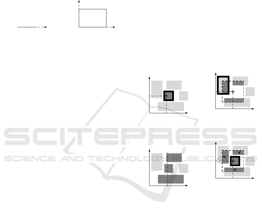
Learning Cycles. During learning cycles, if the
perceptions P
n
belong to the validity ranges of an ex-
isting Context Agent, it is a Valid Context Agent (Fig.
2a). It proposes a prediction with its model. If there
are several Valid Context Agents, the prediction of the
one with the best confidence is retained. It is called
the Best Context Agent for the current execution cy-
cle. If it gives a good prediction, it increments its
confidence. If the prediction is bad all Valid Context
Agents reorganize themselves by following adaptive
behaviors. To know if the prediction of a Context
Agent is good or bad, an error margin and an inac-
curacy margin are used. They are given by the user of
the learning mechanism. A prediction is good if the
error with the oracle’s prediction O
1
is less than the
inaccuracy margin.
Exploitation Cycles. During the exploitation, if
they are several Valid Context Agents, the one with
the higher confidence is the Best Context Agent. It
provides the prediction output O
0
1
. If there aren’t any
Valid Context Agents, the closest Context Agent to the
perceptions is designated as the Best Context Agent.
Shortcomings. The presented rules suffer from a
lack of local interactions between the Context Agents.
This approach proposes a distributed learning method
that is adaptive with respect to the oracle values but
not between the knowledge fragments. Another is-
sue is the scalability of the local added interactions.
AMOEBA does not possess any mechanism allowing
Context Agents to communicate locally without acti-
vating all the Context Agent of the system.
p
1
p
2
(a) Valid Context Agent
with all perceptions.
p
1
p
2
(b) Closest Context Agent
with all perceptions in the
neighborhood.
p
1
p
2
(c) Valid Context Agents on
exploitation with only the
perception p
1
.
p
1
p
2
(d) Cooperative neighbor-
hood learning situations;
the endogenous learning
situations are represented
with diagonal crosses.
Figure 2: Context Agents Mechanisms; Best Context Agent,
valid Context Agents and neighborhood areas are filled
darker; Best Context Agents are boxed; the neighborhood
is represented by a dotted box.
3 ENDOGENOUS CONTEXT
LEARNING
Endogenous Context Learning is an enhancement of
Context Learning using internal information to self-
generate new learning situations. In the next sec-
tions, we differentiate exogenous learning situations
and endogenous learning situations which are re-
spectively provided by an external entity and self-
ICAART 2021 - 13th International Conference on Agents and Artificial Intelligence
370

x
y
x
T
y
T
θ
1
θ
2
θ
3
l
l
Figure 3: 3 joints robotic arm
with segments of equal length l
in a 2D task space.
Figure 4: Explo-
ration with a 3 joints
robotic arm simulation
after 1000 training
situations.
generated by the learning mechanism. This mecha-
nism is based on a collaboration inside the neighbor-
hood of the Context Agents. The presented process is
operational regardless of the number of dimensions.
3.1 Neighborhood
A Context Agent is considered as a neighbor of the
perceptions if its validity ranges intersect a neighbor-
hood area surrounding the current perceptions. The
size of this area results from the precision range, a
parameter chosen by the user of the learning mech-
anism. For a perception p
i
, there is a default ra-
dius creation for a Context Agent r
creation
i
= (p
max
i
−
p
min
i
).precision range. p
max
i
and p
min
i
are the maxi-
mum and minimum experienced values by the learn-
ing mechanism on the perception p
i
. From this,
it results an approximation error distance d
aed
i
=
0.25.r
creation
i
. The neighborhood area radius is r
N
i
=
k
N
.r
creation
i
.
3.2 Endogenous Learning Rules
To take advantage of the neighborhood in the learn-
ing process, it is necessary to modify the rules of
AMOEBA. The inaccuracy margin is removed so
there is only an error margin chosen by the user of
the learning mechanism to define its accuracy expec-
tations.
Bad Prediction Situation. The distance to the
learning situation is greater than the error margin.
The Context Agent is not valid for this learning sit-
uation. Its prediction is not accurate enough given
expected precision. It moves one of its ranges to ex-
clude the current perception and it decreases its con-
fidence. It always chooses the range that least affects
the volume of its validity ranges. If the distance to the
learning situation is less than the error margin, the
agent’s confidence increases and it updates its model
with the current learning situation. There is only one
margin to define whether a Context Agent is good or
bad. The agents’ models are regularly updated to be
robust to noise.
Uselessness Situation. A Context Agent is useless
if one of its validity ranges has a critical size below
d
aed
i
.
Unproductive Situation. The mechanism of ex-
tending the closest good Context Agent remains the
same. The closest good Context Agent extends one of
its ranges towards the new situation. The novelty ap-
pears at the creation of a new Context Agent if needed.
If there are neighbors, they are used to initialize the
properties of the new agent. If there are no neighbors,
the created agent uses initialization values based on
the perception limits of the search space and on the
parameters chosen by the system user.
3.3 Cooperative Neighborhood
Learning
In order to enhance the learning process, each Best
Context Agent communicates with its neighbors to
ask them for endogenous learning situations L
endo
n
=
[P
endo
n
,O
endo
1
]. This has for objective to locally
smooth the models between them. As for the percep-
tion neighborhood radiuses, the prediction neighbor-
hood radius is defined as it follows r
N
O
1
= k
N
.(O
max
1
−
O
min
1
).precision range. The perceptions P
endo
n
of the
endogenous learning situation are chosen randomly
in the intersection of the neighborhood and the neigh-
bor’s validity ranges (fig. 2d). The prediction O
endo
1
is asked to the model of the neighbor. Only neighbors
that have a close last prediction share an endogenous
learning situation. If the difference between the en-
dogenous prediction and the last Best Context Agent
prediction |O
endo
1
−o
Best Context Agent
1,last
| is lesser than r
N
O
1
,
the endogenous learning situations is retained. The
set of all retained endogenous learning situations is
used to update the Best Context Agent model with a
weight w
endo
. To satisfy this weight, artificial Learn-
ing Situations are generated. They are distributed on
the current model according to a normal law centered
in the validity ranges center and with a standard devi-
ation of ((r
j
i,end
− r
j
i,start
)/10)
1
2
. This distribution en-
sures that the center of the model, is slightly altered.
The endogenous learning situations are then used to
estimate new regression parameters using Miller’s re-
gression (Miller, 1992).
Cooperative Neighborhood Learning: Application to Robotic Inverse Model
371

3.4 Context Exploitation
The addition of the neighborhood is useful to opti-
mize the exploitation, specially when there aren’t any
valid Context Agents. In this case, the Best Context
Agent is the closest Context Agent to the perceptions
among the Context Agents neighbors (Fig. 2b). If
they are no neighbors, it is the closest Context Agent
among all the Context Agents. The neighborhood
speeds up the exploitation when there are neighbors
and a lot of Context Agents in the whole system.
In the case that all the perceptions are not provided
for the exploitation, we propose a new way of exploit-
ing the models. The given subset of perceptions is
used to define the set of valid Context Agents. The
Best Context Agent is then chosen using the distance
to the sub-perceptions. The unspecified perceptions
are set by default to the center of the validity ranges
of the Best Context Agent. Fig. 2c shows an exploita-
tion with the sub-perception p
1
only.
4 INVERSE KINEMATICS
LEARNING CASE STUDY
For our experimentations, we repeat one of the ex-
perimental setups of Baranes and Oudeyer (Baranes
and Oudeyer, 2013) which is the learning of the in-
verse kinematics with a redundant arm. We consider
a robotic arm with segments of equal length and n
joints in a 2D plane: (θ
1
,θ
i
,. .. ,θ
n
) (Fig. 3 shows an
example for 3 joints). To control it, one must use its
Forward Kinematic Model FKM and its Inverse Kine-
matic Model IKM which are both non linear models
dependent on the characteristics of the arm. The For-
ward Kinematic Model is used to calculate the po-
sition of the robot tool in a task space from the an-
gles of each joint: FKM(θ
1
,θ
i
,. .. ,θ
n
) = (x
T
,y
T
) for
a task space of two dimensions. The analytical In-
verse Kinematic Model gives all the possible angle
vectors for a desired tool position: IKM(x
T
,y
T
) =
(θ
1
,θ
i
,. .. ,θ
n
),(θ
1
,θ
i
,. .. ,θ
n
)
0
,. ..
We propose here to learn the IKM using the FKM
as a supervisor and to exploit the learning without us-
ing all the Perceptions. This approach is independent
of the joints number of the considered robots.
Training. The training is made from several ran-
dom joints configurations (θ
rdn
1
,θ
rdn
i
,. .. ,θ
rdn
n
). The
corresponding position of the end of the robot
arm is given by the Forward Kinematic Model :
FKM(θ
rdn
1
,θ
rdn
i
,. .. ,θ
rdn
n
) = (x
rdn
T
,y
rdn
T
). The per-
ceptions for the learning mechanism are the po-
sition of the end of the robot (x
rdn
T
,y
rdn
T
) and
all the corresponding angles except the last one
(θ
rdn
1
,θ
rdn
i
,. .. ,θ
rdn
n−1
). The perceptions vector is
(x
rdn
T
,y
rdn
T
,θ
rdn
1
,θ
rdn
i
,. .. ,θ
rdn
n−1
). The last angle θ
rdn
n
is the prediction of the local models. The
global function that is learnt by the mechanism
is F
θ
n
(x
rdn
T
,y
rdn
T
,θ
rdn
1
,θ
rdn
i
,. .. ,θ
rdn
n−1
) = θ
rdn
n
. We
define the training learning situations as exoge-
nous learning situations given by the joints con-
figuration of the robot and its FKM: L
exo
n
=
[(x
rdn
T
,y
rdn
T
,θ
rdn
1
,θ
rdn
i
,. .. ,θ
rdn
n−1
),θ
rdn
n
].
Exploration. The generation of the random angles
for the joints is done following a normal distribution.
Considering that an outstretched arm is defined by
all the angles being set to 0 rad, the distribution of
each angle is centered around this value except for θ
1
which has an homogeneous random distribution be-
tween 0 and 2π. The dispersion is set empirically for
3, 10 and 30 joints with the objective of having ho-
mogeneous situations in the task space (Fig. 4 shows
an example of exploration with 3 joints after 1000 ex-
ogenous learning situations). The obtained dispersion
depending on the number of joints is : 2.5593n
−0.479
.
Exploitation. As we are learning the IKM, the goal
here is to get a set of angles to position the end of
the robotic arm in a point P
goal
xy
= (x
goal
T
,y
goal
T
) (fig.
3). All P
goal
xy
are randomly generated in the reach-
able zone of the task space. It is an exploitation
without all the perceptions and the sub-perceptions
are x
goal
T
and y
goal
T
. The learning mechanism is given
(x
goal
T
,y
goal
T
) and it provides a joints configuration
(θ
explo
1
,θ
explo
i
,. .. ,θ
explo
n
).
5 EXPERIMENTATIONS
In this section, we present our results achieved with
the addition of endogenous leaning situations in the
learning of robotic arms inverse models. A learning
cycle corresponds to a configuration for the robotic
arm. The learning mechanism receives an exogenous
learning situation at each learning cycle. The inverse
models to be learnt are non linear models of high di-
mensions (up to 30). We chose to stop at 30 to match
the numbers of degrees of freedom on a usual hu-
manoid robot. We are aware that on a humanoid all
linkages are not serial. The goal here is to test our
approach with the same degrees of freedom order of
magnitude.
ICAART 2021 - 13th International Conference on Agents and Artificial Intelligence
372
5.1 Metrics
Goal Error. To appraise the score of the learnt IKM,
we evaluate the proposals of the learning mechanism.
We calculate the end position error of the robot in the
task space E
T
. This error is the distance between the
randomly asked positions P
goal
xy
in the reachable task
space and the position resulting from the exploitation
of the learning P
explo
xy
. This error is normalized by
the diameter of the reachable space D
reachable
which
is a disk in this case: E
T
= ||
# »
P
goal
xy
P
explo
xy
||/D
reachable
.
The prediction metric is calculated over exploitation
cycles where the mechanism is asked to make angles
predictions to get the goal position.
Endogenous Data. To evaluate the impact of the
cooperative neighborhood mechanism on the goal
performances, we are interested in the number of gen-
erated endogenous learning situations L
endo
n
.
5.2 Results
The presented results are averaged over 15 learning
experiences. Each learning experience is stopped af-
ter 1000 training cycles. The goal errors are av-
eraged over 200 exploitation cycles. The stretched
length for each tested arms is the same (50 units in
our simulation). Each arm segment is the same size.
For each arm size scenario, the size of the reachable
space is the same. The error margin is set to 1. The
weight w
endo
of endogenous learning situations is 0.1.
The code is implemented in java with the framework
AMAK (Perles et al., 2018) and it is executed on a
machine
1
with Ubuntu 18.04.3 LTS.
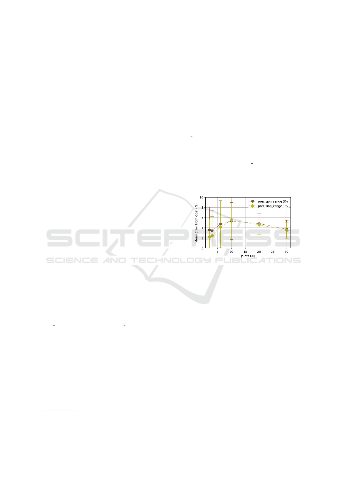
Arm Dimensions. Figure 5 shows that without
cooperative neighborhood learning the best perfor-
mance is obtained for 2 joints and with a preci-
sion range of 1%. The precision range of 1% also
gives lower mean error for the arms of 2, 3 and 6 joints
than the precision range of 3%. For arms with more
joints the gap is less visible. We can also see that the
mean error and its dispersion increase up to 10 joints.
Then, they decrease as the number of joints gets big-
ger.
Neighborhood Sizes. Figure 6 shows that the size
of the neighborhood has an impact on the mean er-
ror for the arms of 2, 3 and 6 joints. With a preci-
sion range of 3% the error decreases and reaches a
1
Intel(R) Core(TM) i7-4790 CPU @ 3.60GHz × 8,
RAM 31.4 GB.
minimum value with a delay in the neighborhood size
for the different arms. It then increases for 2 and 3
joints for high neighborhood sizes. For 10, 20 and 30
joints (Fig. 7), the error only decreases for 10 joints.
The other cases are not impacted by the variation of
neighborhood.
Endogenous Data. Figures 8 and 9 represent the
same experimentation than 6 and 7 but focusing on
the variation of the error according to the endogenous
learning situations. Fig. 8, for 6 joints and a preci-
sion range of 3%, the more endogenous learning sit-
uations there are, the lower the error is. For 2 and 3
joints, we find the same behavior than Fig. 6, there is
an optimal situation beyond which the error increases.
For 10 joints with a precision range of 3% (Fig. 9),
more endogenous learning situations reduce the error.
But for 20 and 30 joints, the endogenous learning sit-
uations don’t reduce the goal error, they even slightly
increase it.
Figure 5: Mean errors from goal depending on robotic arm
sizes (2, 3, 6, 10, 20 and 30 joints) without cooperative
neighborhood learning. Learning cycles = 1000; exploita-
tion cycles = 200; averaged overs 15 learning experiences.
5.3 Discussion
We have seen that the lowest error is obtained for the
lowest arm dimensions. The error increases up to 10
joints and it decreases for higher arm dimensions. At
low dimensions, the good performance is due to the
low redundancy of the problem making the explo-
ration less extensive. The decreasing of the error at
high dimensions is caused by the exploitation of the
Context Agents with sub-perceptions. If the requested
goal P
goal
xy
during the exploitation is in a less explored
area, it is the closest model that is used for the last
angle prediction. The smaller the size of the last arm
segment, the smaller the distance error on the goal.
Which is the case for the higher dimensions. The rest
of the angles are fixed using the validity ranges of the
Best Context Agent.
Figures 6, 7, 8 and 9 showed that the expansion
of the neighborhood can lead to better or worse per-
Cooperative Neighborhood Learning: Application to Robotic Inverse Model
373
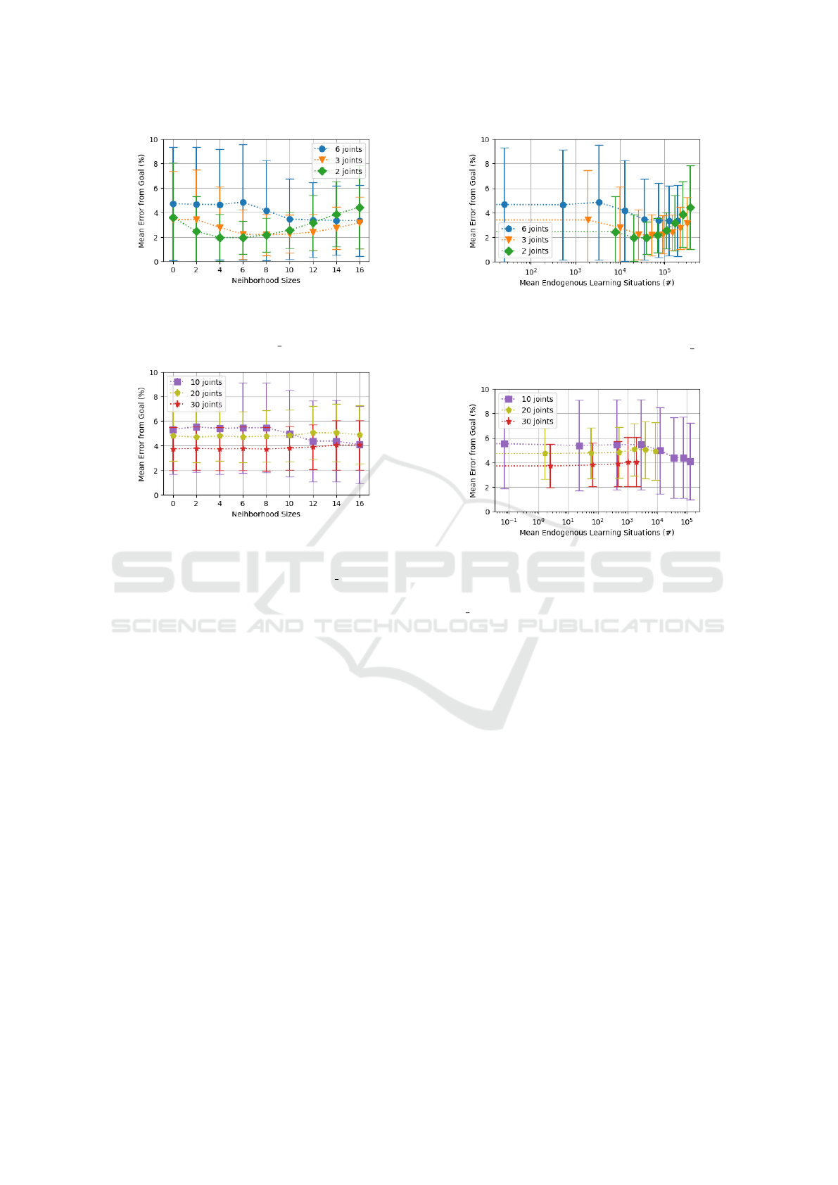
Figure 6: Mean errors from goal depending on mean neigh-
borhood sizes over robotic arms of 2,3 and 6 joints. Learn-
ing cycles = 1000; exploitation cycles = 200; averaged overs
15 learning experiences. precision range = 3%.
Figure 7: Mean errors from goal depending on mean neigh-
borhood sizes over robotic arms of 10,20 and 30 joints.
Learning cycles = 1000; exploitation cycles = 200; aver-
aged overs 15 learning experiences. precision range = 3%.
formances by generating more endogenous learning
situation. The point of best performance is different
for each arm sizes which shows that the neighborhood
behaves differently with higher dimensions. Past this
point, the error increases because the endogenous
learning situations are too far from the Context Agent
to bring a coherent smoothing. At high dimensions,
endogenous learning situations are harder to gener-
ate because of the large exploration space. This is
why, for the same neighborhood sizes, there are more
endogenous learning situations at low dimensions.
Moreover, beyond 10 joints, the performances are not
affected by the endogenous learning situation.
5.3.1 Related Work
The magnitude of the mean goal reaching errors of
the Self-Adaptive Goal Generation RIAC algorithm
(SAGG-RIAC) (Baranes and Oudeyer, 2013) is close
to our results. The difference is that SAGG-RIAC
uses around 10
4
micro actions for each goal to ob-
tain comparable goal errors. Our approach instanta-
neously gives a set of angles to reach any goal after
one training of 1000 learning situations.
Figure 8: Mean errors from goal depending on mean en-
dogenous learning situations over robotic arms of 2, 3 and
6 joints. Learning cycles = 1000; exploitation cycles = 200;
averaged overs 15 learning experiences. precision range =
3%.
Figure 9: Mean errors from goal depending on mean en-
dogenous learning situations over robotic arms of 10, 20
and 30 joints. Learning cycles = 1000; exploitation cy-
cles = 200; averaged overs 15 learning experiences; pre-
cision range = 3%.
6 CONCLUSION AND
PERSPECTIVES
In this paper, we have proposed an extension of a
Context-based learning multi-agent system which has
already proven to be suitable to complex systems
and that is directly inspired by Constructivism. This
is a generic approach because it does not rely on
the underlying application. This work was applied
on the learning of the Inverse Kinematic Models of
robotic arms with different numbers of joints. Self-
observation of self-adaptive multiagent systems al-
lowed us to add collaboration between fragments of
learning which are the Context Agents. Based on
the internal detection of close Context Agents models,
we proposed the generation of endogenous learning
situations that led to better performances on Inverse
Kinematic Model learning. This work has shown
that the generation of endogenous learning situations
makes it possible to reduce exogenous learning situ-
ations as the performance improvement with endoge-
nous cooperative learning attests.
ICAART 2021 - 13th International Conference on Agents and Artificial Intelligence
374

The proposed approach needs to be refined in or-
der to select the right size of neighborhood accord-
ing to the dimension of the exploring space to maxi-
mize performance. The scalability was not discussed
here but the generation of endogenous learning situ-
ations at high dimensions needs also to be optimized
to access to more neighbors with reasonable execu-
tion times. Another promising lead is to decompose
the learning into several local instances of the learn-
ing mechanism, one for each joint. This would re-
duce the high-dimensional problem into several low-
dimensional problems where the cooperative neigh-
borhood learning is more effective. It will also ensure
that the performances are independent of the number
of dimensions, and that the execution time is linearly
dependent on the dimensions.
REFERENCES
Aristidou, A., Lasenby, J., Chrysanthou, Y., and Shamir,
A. (2018). Inverse kinematics techniques in computer
graphics: A survey. In Computer Graphics Forum,
volume 37, pages 35–58. Wiley Online Library.
Ashby, W. R. (1956). Cybernetics and requisite variety. An
Introduction to Cybernetics.
Baranes, A. and Oudeyer, P.-Y. (2013). Active learning of
inverse models with intrinsically motivated goal ex-
ploration in robots. Robotics and Autonomous Sys-
tems, 61(1):49–73.
Bayle, B., Fourquet, J.-Y., and Renaud, M. (2003). Manipu-
lability of wheeled mobile manipulators: Application
to motion generation. The International Journal of
Robotics Research, 22(7-8):565–581.
Boes, J., Nigon, J., Verstaevel, N., Gleizes, M.-P., and Mi-
geon, F. (2015). The self-adaptive context learning
pattern: Overview and proposal. In International and
Interdisciplinary Conference on Modeling and Using
Context, pages 91–104. Springer.
Chaput, H. H. (2004). The constructivist learning archi-
tecture: A model of cognitive development for robust
autonomous robots. PhD thesis.
Drescher, G. L. (1991). Made-up minds: a constructivist
approach to artificial intelligence. MIT press.
Ferber, J. (1999). Multi-agent systems: an introduction to
distributed artificial intelligence, volume 1. Addison-
Wesley Reading.
Georg
´
e, J.-P., Gleizes, M.-P., and Camps, V. (2011). Coop-
eration. In Self-organising Software, pages 193–226.
Springer.
Gu
´
eriau, M., Armetta, F., Hassas, S., Billot, R., and
El Faouzi, N.-E. (2016). A constructivist approach for
a self-adaptive decision-making system: application
to road traffic control. In 2016 IEEE 28th Interna-
tional Conference on Tools with Artificial Intelligence
(ICTAI), pages 670–677. IEEE.
Guerin, F. (2011). Learning like a baby: a survey of arti-
ficial intelligence approaches. The Knowledge Engi-
neering Review, 26(2):209–236.
Ho, E. S., Shum, H. P., Cheung, Y.-m., and Yuen, P. C.
(2013). Topology aware data-driven inverse kinemat-
ics. In Computer Graphics Forum, volume 32, pages
61–70. Wiley Online Library.
Holden, D., Saito, J., and Komura, T. (2016). A deep
learning framework for character motion synthesis
and editing. ACM Transactions on Graphics (TOG),
35(4):1–11.
Holmes, M. P. et al. (2005). Schema learning: Experience-
based construction of predictive action models. In
Advances in Neural Information Processing Systems,
pages 585–592.
Hootsmans, N. and Dubowsky, S. (1991). Large motion
control of mobile manipulators including vehicle sus-
pension characteristics. In ICRA, volume 91, pages
2336–2341.
Jamali, A., Khan, R., and Rahman, M. M. (2011). A new
geometrical approach to solve inverse kinematics of
hyper redundant robots with variable link length. In
2011 4th International Conference on Mechatronics
(ICOM), pages 1–5. IEEE.
Kearns, M. J., Schapire, R. E., and Sellie, L. M. (1994). To-
ward efficient agnostic learning. Machine Learning,
17(2-3):115–141.
Mazac, S., Armetta, F., and Hassas, S. (2014). On boot-
strapping sensori-motor patterns for a constructivist
learning system in continuous environments. In Artifi-
cial Life Conference Proceedings 14, pages 160–167.
MIT Press.
Miller, A. J. (1992). Algorithm as 274: Least squares rou-
tines to supplement those of gentleman. Journal of the
Royal Statistical Society. Series C (Applied Statistics),
41(2):458–478.
Nigon, J., Gleizes, M.-P., and Migeon, F. (2016). Self-
adaptive model generation for ambient systems. Pro-
cedia Computer Science, 83:675–679.
Oudeyer, P.-Y. et al. (2014). Socially guided intrinsic moti-
vation for robot learning of motor skills. Autonomous
Robots, 36(3):273–294.
Perles, A., Crasnier, F., and Georg
´
e, J.-P. (2018). Amak-
a framework for developing robust and open adaptive
multi-agent systems. In International Conference on
Practical Applications of Agents and Multi-Agent Sys-
tems, pages 468–479. Springer.
Perotto, F. S. (2013). A computational constructivist model
as an anticipatory learning mechanism for coupled
agent–environment systems. Constructivist Founda-
tions, 9(1):46–56.
Piaget, J. (1976). Piaget’s theory. Springer.
Provost, J., Kuipers, B. J., and Miikkulainen, R. (2006). De-
veloping navigation behavior through self-organizing
distinctive-state abstraction. Connection Science,
18(2):159–172.
Thuruthel, T. G., Falotico, E., Cianchetti, M., and Laschi, C.
(2016). Learning global inverse kinematics solutions
for a continuum robot. In Symposium on Robot De-
sign, Dynamics and Control, pages 47–54. Springer.
Unzueta, L., Peinado, M., Boulic, R., and Suescun,
´
A. (2008). Full-body performance animation with
sequential inverse kinematics. Graphical models,
70(5):87–104.
Cooperative Neighborhood Learning: Application to Robotic Inverse Model
375
