Using Anatomical Priors for Deep 3D One-shot Segmentation

Duc Duy Pham, Gurbandurdy Dovletov and Josef Pauli

Intelligent Systems, Faculty of Engineering, University of Duisburg-Essen, Germany

Keywords:

Shape Priors, Anatomical Priors, One-shot Segmentation.

Abstract:

With the success of deep convolutional neural networks for semantic segmentation in the medical imaging

domain, there is a high demand for labeled training data, that is often not available or expensive to acquire.

Training with little data usually leads to overﬁtting, which prohibits the model to generalize to unseen prob-

lems. However, in the medical imaging setting, image perspectives and anatomical topology do not vary as

much as in natural images, as the patient is often instructed to hold a speciﬁc posture to follow a standardized

protocol. In this work we therefore investigate the one-shot segmentation capabilities of a standard 3D U-Net

architecture in such setting and propose incorporating anatomical priors to increase the segmentation perfor-

mance. We evaluate our proposed method on the example of liver segmentation in abdominal CT volumes.

1 INTRODUCTION

In medical image computing, semantic segmentation

of anatomical structures from various imaging modal-

ities is a crucial task to aid in image based diagnostics.

Therefore, research on automated segmentation meth-

ods is a major topic in the medical computing domain,

since manual segmentation is expensive and time con-

suming. Especially deep learning strategies have be-

come popular approaches to achieve state of the art re-

sults. Ronneberger et al.’s U-Net (Ronneberger et al.,

2015) has achieved a lot of attention, yielding impres-

sive results in many medical applications. While its

general architecture has been modiﬁed in numerous

ways, (Isensee et al., 2018) demonstrate the effec-

tiveness of a well trained U-Net without substantial

architectural modiﬁcations in the BraTS 2018 chal-

lenge. Therefore, the U-Net architecture has become

a competitive baseline for state of the art segmenta-

tion performance. However, it does not take into con-

sideration the low variation in shape for most anatom-

ical structures. Consequently, recent research aims at

incorporating shape priors into the segmentation pro-

cess. (Ravishankar et al., 2017) propose augmenting

the U-Net by means of a pre-trained autoencoder that

is used for shape regularization. The U-Net’s output

is corrected by the autoencoder to result in a feasible

shape. (Oktay et al., 2018) also utilize a pre-trained

autoencoder for shape preservation. However, the au-

toencoder’s encoding component is used to regularize

the weight adaptation process of a generic segmenta-

tion network during training, instead of merely cor-

recting the initial segmentation output. This is moti-

vated by (Girdhar et al., 2016)’s work on establish-

ing 3D representations of objects from 2D images.

(Dalca et al., 2018) take into consideration shape pri-

ors by means of pre-trained variational autoencoders

for an unsupervised learning scheme. (Pham et al.,

2019) present a 2D end-to-end architecture, in which

an autoencoder, trained for shape representation, is

imitated in latent space by a separate encoder, to di-

rectly leverage the autoencoder’s decoder for shape

consistent segmentation.

A limiting factor for most deep learning strategies is

the amount of data needed to sufﬁciently train deep

learning models. Especially in the medical domain,

labeled training data is scarce and expensive to ac-

quire. As a result, one-shot and few-shot learning ap-

proaches have been developed for classiﬁcation tasks

in natural image settings (Koch et al., 2015; Santoro

et al., 2016; Snell et al., 2017; Vinyals et al., 2016).

There is, however, little research towards one-shot

and few-shot learning for segmentation tasks, e.g. by

(Dong and Xing, 2018; Michaelis et al., 2018), par-

ticularly for medical images, e.g. (Roy et al., 2020).

While distinguishing between tissue classes can be

more challenging than in natural images, medical im-

ages are usually more constrained regarding perspec-

tive and shapes. Our contributions are the following:

• We examine to which extend a 3D U-Net archi-

tecture is capable of segmenting unseen volumes

in a one-shot segmentation setting.

• We compare its results to architectures that make

174

Pham, D., Dovletov, G. and Pauli, J.

Using Anatomical Priors for Deep 3D One-shot Segmentation.

DOI: 10.5220/0010303101740181

In Proceedings of the 14th International Joint Conference on Biomedical Engineering Systems and Technologies (BIOSTEC 2021) - Volume 2: BIOIMAGING, pages 174-181

ISBN: 978-989-758-490-9

use of additional anatomical priors.

• We present and investigate an architecture of our

own, which can be regarded as a combination of

(Pham et al., 2019)’s and (Oktay et al., 2018)’s

work.

2 METHODS

Motivated by(Oktay et al., 2018)’s contribution and

based on (Pham et al., 2019)’s work regarding

anatomical priors, we investigate a combined 3D seg-

mentation approach in a one-shot setting. We propose

a 3D end-to-end Imitating and Regularizing Encoders

and Enhanced Decoder Network (IRE

D-Net) that is

derived from the IE

D-Net, leveraging Oktay et al.’s

enforcement of stronger shape regularization. The

architecture consists of two convolutional encoders

enc

, f

enc

, one decoder g

dec

and one U-Net compo-

nent h

unet

as depicted in Fig. 1. While f

enc

and

dec

form a convolutional autoencoder (CAE), f

enc

and g

dec

constitute a segmentation hourglass network.

The standard U-Net module h

unet

is used to enhance

dec

for an image guided decoding process to increase

the decoder’s localization capabilities. Additionally,

enc

serves as a regularization module, that measures

the output’s shape consistency in latent space during

training.

2.1 Enforcing Shape Preservation

Convolutional autoencoders are able to both compress

their input into a meaningful representation in latent

space, and reconstruct the original input from this rep-

resentation with only little to none information loss.

We leverage this property to inject prior information

into the learning process of a deep learning network.

In our architecture we use the mapping from input to

latent feature space for two strategies of shape preser-

vation. On the one hand, we employ (Girdhar et al.,

2016)’s approach of imitating the autoencoder’s prior

encoder f

enc

in latent space by an additional imitat-

ing encoder f

enc

, that infers the actual medical vol-

ume instead of the ground truth volume. We denote

the input volume as x and the segmentation ground

truth as y, and Θ represents the trainable weights of

the architecture. Then the mapping of y into latent

space is

ˆz = f

enc

(y, Θ

enc

), (1)

whereas the imitation in latent space from x is

˜z = f

enc

(x, Θ

enc

). (2)

The formulation of an imitation loss

imit

(Θ

enc

|Θ

enc

) := ||ˆz − ˜z||

, (3)

where Θ

enc

is adaptable and Θ

enc

is ﬁxed, enforces

enc

to encode the input volume in a similar fashion

to f

enc

during training. The idea is to utilize the au-

toencoder’s decoder g

dec

to achieve a segmentation

˜y = g

dec

( f

enc

(x, Θ

enc

), Θ

dec

) (4)

from x that is close to the ground truth y. Further-

more, the decoder receives skip connections from the

U-Net’s contracting path, enhancing the decoder’s lo-

calization capabilities.

On the other hand, we additionally leverage f

enc

restrain the output segmentation’s shape by compar-

ing its latent representation to the ground truth’s, em-

ploying a shape consistency loss

(Θ

enc

, Θ

dec

, Θ

unet

|Θ

enc

) :=



enc



˜y + h

unet

(x)



− f

enc

(y)



, (5)

which is used to adapt Θ

enc

, Θ

dec

and Θ

unet

, whereas

enc

is kept ﬁxed. Like (Oktay et al., 2018) we add

this loss as a regularizing term to the segmentation

losses of the segmentation networks. Inclined by the

success of ensemble methods, the output of the U-Net

module is ﬁnally added to the segmentation output

from the imitating hourglass network in a component-

wise manner.

2.2 Differences in Training and

Inference

As can be seen in Fig.1, our architecture consists

of two segmentation networks, i.e. the U-Net mod-

ule and the hourglass network module. Even though

the hourglass network’s decoder receives skip con-

nections from the U-Net’s contracting path, both ar-

chitectures are optimized separately using the Dice

Loss and regularized by L

, weighted by a factor λ.

The autoencoder is also trained separately from the

segmentation networks by means of the Dice Loss.

The imitating encoder is optimized by the aforemen-

tioned imitation loss L

imit

. During training, the prior

encoder’s main purpose is to deliver a reference for

the imitation encoder to compare against. Since f

enc

needs a ground truth segmentation as input, it is es-

sentially replaced by f

enc

that is trained to map med-

ical images to a similar feature in latent space. Also,

shape consistency regularization is only possible dur-

ing training, therefore f

enc

is omitted during infer-

ence.

Using Anatomical Priors for Deep 3D One-shot Segmentation

175

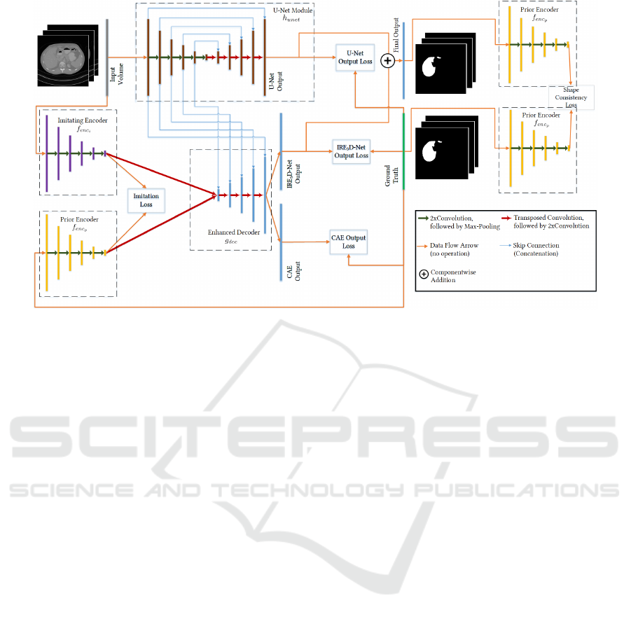
Figure 1: Network Architecture. The architecture consists of four modules: the U-Net module (brown), the imitating encoder

(purple), the prior encoder (yellow), and the joint decoder (blue). The prior encoder is additionally used for shape consistency

of the output segmentation and the ground truth. For inference the prior encoder is omitted.

3 EXPERIMENTS

3.1 Data

We evaluated on the example of liver segmentation

from abdominal CT volumes, using both the Cancer

Imaging Archive Pancreas-CT data set (Clark et al.,

2013; Roth et al., 2016; Roth et al., 2015) (TCIA)

and the Beyond the Cranial Vault (BTCV) segmenta-

tion challenge (Landman et al., 2015; Xu et al., 2016)

with supplementary ground truth segmentations pro-

vided by (Gibson et al., 2018), resulting in ninety

abdominal CT volumes with corresponding ground

truths in total. Since we examine the one-shot ca-

pability of a standard U-Net implementation and the

effect of incorporating anatomical priors into a deep

learning architecture, the U-Net model, (Oktay et al.,

2018)’s ACNN , (Pham et al., 2019)’s IE

D and our

newly proposed IRE

D are all trained with only one

patient data set for each test scenario. In an exhaustive

leave-one-out cross validation manner, we trained ev-

ery architecture 90 times, using each patient data set

as one-shot training set once, and tested on the re-

maining patient data sets, that have not been involved

in training or validation. We arbitrarily used patients

40 and 90 as validation data sets. When training with

patient 40 we used patients 39 and 90 for validation

and when training with patient 90, we used patients 40

and 89 for validation. We considered the commonly

used Dice Similarity Coefﬁcient (DSC) and the Haus-

dorff Distance (HD) as evaluation metrics. While the

DSC is a similarity measure between ground truth and

prediction, the HD measures the distance to the fur-

thest falsely classiﬁed voxel. As a reference (Ref)

we calculated the DSC for each test data set, which

is achieved by just regarding the ground truth of the

training data set as ﬁnal segmentation for the test sets.

We additionally simulate a Situs Inversus case, in

which the organs are ﬂipped. This is motivated by

our intention to investigate how the trained networks

react to cases that slightly differ from physiological

images obtained in the usual standard scanning pro-

cedure. We do so by inverting the stack ordering in

longitudinal axis for validation and all test data sets,

while keeping the ordering for the training set.

3.2 Implementation Details

We resized the CT volumes to an input size of 128 ×

128 × 96 and used Tensorﬂow 1.12.0 for our network

implementations. For all models, and for all the sep-

arately trainable modules, the optimization was per-

formed with an Adam Optimizer with an initial learn-

ing rate of 0.001. The training volume was aug-

mented by means of random translation and rotation.

With a batch size of 1, we trained each model for

2400 iterations and chose the model with best valida-

tion loss for evaluation. Starting with 32 kernels for

each convolutional layer in the ﬁrst resolution level of

each encoder/contracting path, we doubled the num-

BIOIMAGING 2021 - 8th International Conference on Bioimaging

176

ber of kernels for each resolution level on the encod-

ing/contracting side and halved the number of kernels

on the expansive/decoding side for each architecture.

We used a kernel size of 3 × 3 × 3 for every convolu-

tional layer and 2 × 2 × 2 max-pooling in each archi-

tecture. The weight of the regularization term in both

the ACNN and the IRE

D was set to λ = 0.001, as

suggested by (Oktay et al., 2018). The experiments

were conducted on a GTX 1080 TI GPU.

4 RESULTS

Since the complete data set origins from two different

sources, we differentiate between 4 cases regarding

evaluation results:

• Q

: Trained on TCIA and tested on TCIA

• Q

: Trained on TCIA and tested on BTCV

• Q

: Trained on BTCV and tested on TCIA

• Q

: Trained on BTCV and tested on BTCV

These four cases are especially noticeable for the ref-

erence DSC measures in Fig.2, where the achieved

DSCs for each train/test patient combination is de-

picted as a heat map. Rows indicate the patient data

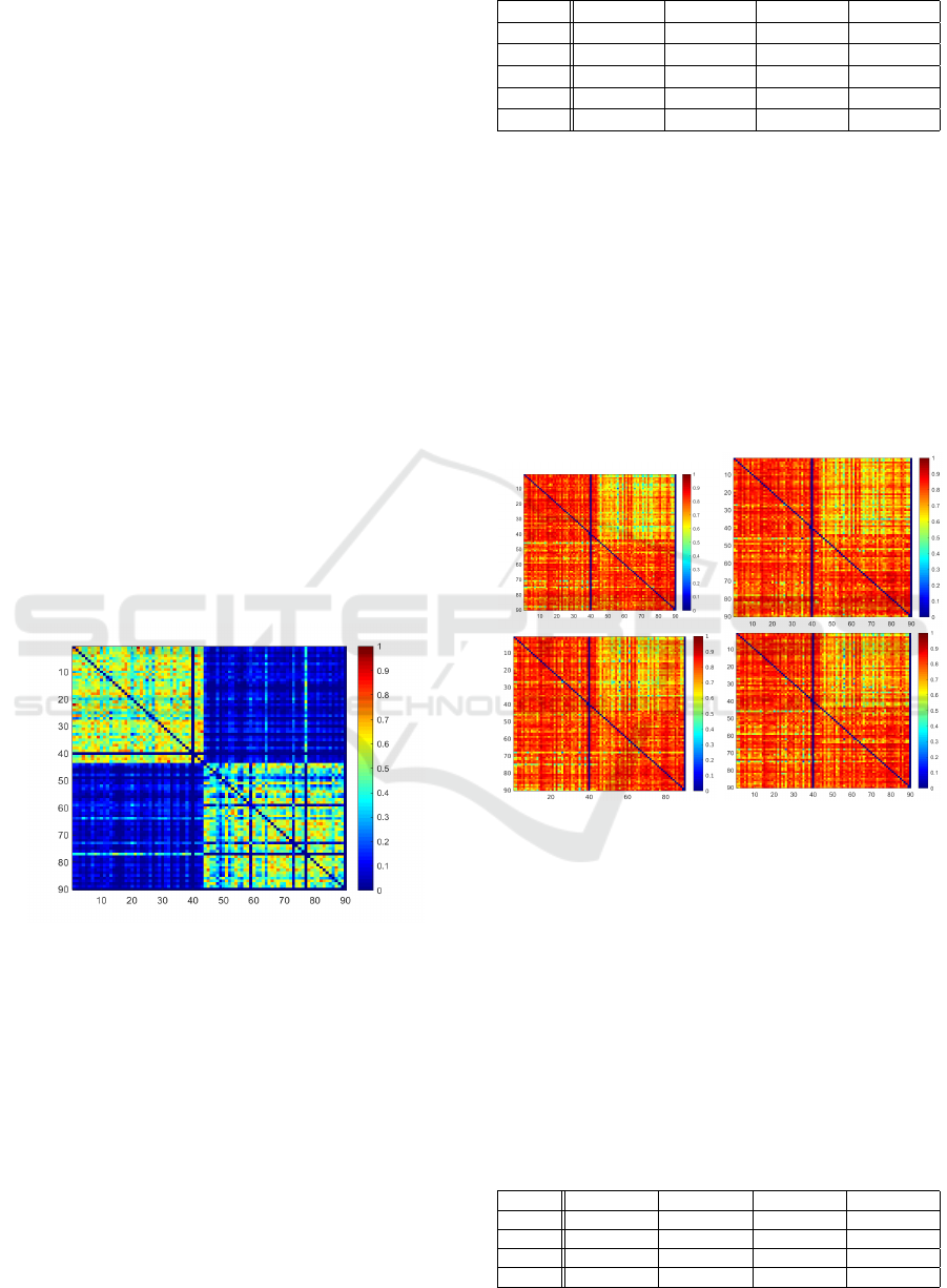
Figure 2: DSC Heatmap of Reference for ordinary setting.

Rows indicate patient used for training, columns represent

test data set.

set used for training, whereas columns represent the

patient test data set. While the columns for patient

40 and 90 are empty, as they serve as validation data

sets, a strong DSC change is visible from column

43 to 44 and row 43 to 44. In particular, the DSCs

get worse, when ground truths come from different

data sources. This indicates that there already is a

strong overlap between ground truths within each data

source. The segmentation problem might therefore be

easier when train and test patients are within the same

data source. This becomes quantitatively visible in

Table 1, in which the resulting mean DSCs for each

Table 1: Achieved DSCs in each case.

DSC Q

Ref 53.7 ± 12 31.7 ± 13 31.7 ± 13 40.7 ± 20

U-Net 82.9±6 67.3 ± 11 78.4 ± 9 80.3±7

ACNN 82.5 ± 6 69.6 ± 10 79.0±8 79.7 ± 8

D 82.1 ± 7 70.2 ± 11 78.4 ± 10 80.3 ± 7

IRE

D 81.8 ± 7 70.5 ±11 77.6 ± 10 80.1 ± 8

architecture in each case are shown.

For the reference and all tested architectures, the

best DSCs are achieved in Q

and Q

. Table 1 also

shows, that the standard U-Net yields the best results

regarding DSC in Q

and Q

, while architectures

with anatomical priors show slightly better results in

and Q

, i.e. when data sources for training and

testing are different. Our proposed IRE

D architec-

ture achieves the best DSC result for the Q

case,

whereas for Q

Oktay et al.’s ACNN surpassed the

remaining models. Fig.3 depicts the DSC heatmaps

of all trained models.

Figure 3: DSC Heatmaps for each train/test combination of

U-Net, ACNN, IE

D, IRE

D (from top left to bottom right)

for ordinary setting. Rows indicate patient used for training,

columns represent test data set.

It becomes visually apparent, that the Q

case

seems to be especially difﬁcult for all models. The ob-

servation that models with shape priors perform bet-

ter when source and target domain are different is,

however, only partly reﬂected by the Hausdorff Dis-

tances in Table 2. Surprisingly, the regularization in

the ACNN results in higher Hausdorff distances than

for the standard U-Net in all cases. Our proposed

IRE

D Network shows best results regarding HD in

Table 2: Achieved HDs in each case.

HD Q

U-Net 50.8 ± 12.9 40.4±11.1 48.6 ± 14.2 48.2±12.7

ACNN 60.1 ± 19.1 45.6 ± 13.3 55.7 ± 23.5 54.8 ± 14.1

D 48.1 ± 13.4 40.5 ± 10.5 45.9 ± 13.1 51.7 ± 12.4

IRE

D 47.8±12.8 40.4 ± 10.7 45.1±12.8 51.1 ± 12.8

Using Anatomical Priors for Deep 3D One-shot Segmentation

177

and Q

, whereas in the challenging Q

case it

preforms equally well as the U-Net. Fig. 4 shows

Figure 4: Hausdorff Distance Heatmaps for each train/test

combination of U-Net, ACNN, IE

D, IRE

D (from top left

to bottom right) for ordinary setting. Rows indicate patient

used for training, columns represent test data set.

the maps of measured Hausdorff distances for each

train/test scenario in each model. Red indicates high

distances wheras blue represents low values. The sur-

prising observation is here visualized, as it can be seen

that the ACNN architecture seems to have difﬁculties

especially in Q

and Q

. While the tested models

with shape prior information and our proposed IRE

model show promising results for one-shot settings in

which source and target domain are different, it is still

surprising that a standard U-Net is also capable of

achieving that good DSC and HD scores when only

training with one data set. Therefore, we would like

to investigate if this observation still holds, when train

and test data show a stronger deviation, such as the Si-

tus Inversus setting.

4.1 Situs Inversus Simulation

In the Situs Inversus setting, it becomes imminent in

the Reference heat map in Fig. 5, that Q

yields the

most challenging case, whereas Q

seems to be the

easiest scenario.

This may be due to the fact, that in BTCV the

liver is not centered along the longitudinal axis. Thus,

when inverting the stack order, the overlap of liver re-

gions between training and testing data set is smaller

than in the other cases. In TCIA, particularly, the liver

is more centered, such that even when inverting the

order, the overlap of liver regions is still rather large.

Table 3 reveals, that the IE

D architecture and our

proposed model outperform the standard U-Net in all

cases except for Q

, where the standard U-Net yields

best DSC results.

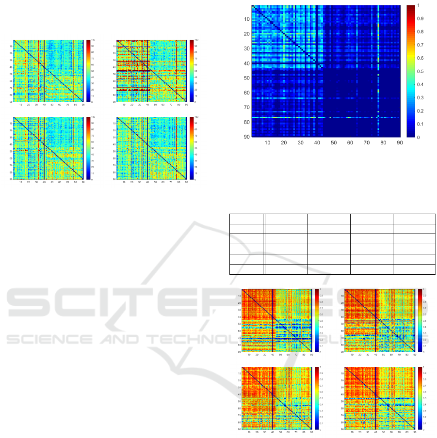
Figure 5: DSC Heatmap of Reference for Situs Inversus

setting . Rows indicate patient used for training, columns

represent test data set.

Table 3: Achieved DSCs in each case for a situs inversus

setting.

Ref 26.0 ± 10 8.3 ± 8 8.3 ± 8 1.4 ± 5

U-Net 76.2±7 59.3 ± 11 60.4 ± 17 45.0 ± 18

ACNN 76.0 ± 7 61.1 ± 11 59.7 ± 19 45.9 ± 18

D 75.4 ± 8 61.8 ± 11 63.7±16 52.4±16

IRE

D 75.8 ± 8 63.0±10 61.9 ± 16 51.2 ± 16

Figure 6: DSC Heatmaps for each train/test combination of

U-Net, ACNN, IE

D, IRE

D (from top left to bottom right)

for situs inversus setting. Rows indicate patient used for

training, columns represent test data set.

Figure 6 shows the DSC heatmaps of the trained

models for each train/test combination. It is di-

rectly noticable that for Q

all models perform very

well, wheras the most problematic case is Q

, i.e.

when there is only little segmentation overlap be-

tween training and testing image. To explore the im-

provements by incorporating shape priors compared

to U-Net we visualize the signed difference maps of

the DSC heatmaps in Fig.7. The ﬁrst column of the

ﬁgure highlights the train/test cases in which U-Net

BIOIMAGING 2021 - 8th International Conference on Bioimaging

178

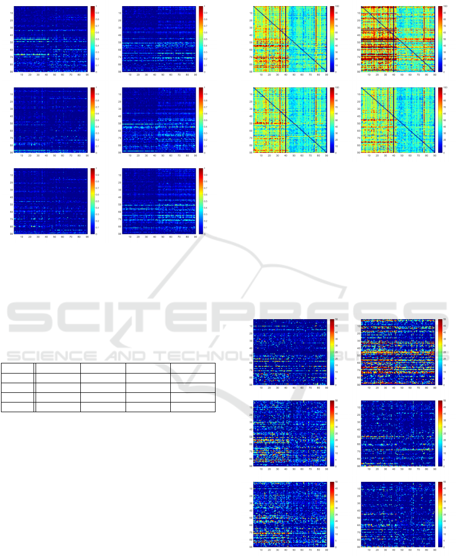
Figure 7: First column: DSC improvement for each

train/test combination, in which U-Net performs better than

ACNN, IE

D, IRE

D for situs inversus setting. Second

column: DSC improvement for each tra(from top to bot-

tom)in/test combinations, in which ACNN, IE

D, IRE

(from top to bottom) perform better than U-Net for situs

inversus setting. Rows indicate patient used for training,

columns represent test data set.

Table 4: Achieved HDs in each case for a situs inversus

setting.

HD Q

U-Net 55.7±12.1 42.0±11.3 60.5±17.8 42.0±11.2

ACNN 64.4±18.0 46.9±14.0 71.9±24.4 51.6±18.0

D 52.3±12.8 40.1±10.6 54.2±15.5 39.6±10.6

IRE

D 51.4±12.3 39.8±10.4 55.2±16.6 39.2±10.3

performs better, whereas the second column shows

the cases in which U-Net preforms worse. We can see

that for IE

D and IRE

D there are many cases, espe-

cially in Q

and Q

, in which U-Net yields inferior

DSC scores. Considering the Hausdorff distances in

Table 4, IE

D and IRE

D also show better results than

the U-Net in all cases. It is, however, surprising that

the shape regularization in ACNN, again, results in

considerably worse Hausdorff distances in all cases.

These observations are visualized in Fig.8, in which

the worse Hausdorff distances of ACNN become im-

mediately apparent in comparison to the other archi-

tectures. As before we would like to compare the

shape prior based models with the standard U-Net

by computing the signed difference in Hausdorff dis-

tances in Fig.9. The left column of the ﬁgure high-

lights in which train/test cases U-Net achieves worse

Hausdorff distances, whereas the right column shows

Figure 8: Hausdorff Distance Heatmaps for each train/test

combination of U-Net, ACNN, IE

D, IRE

D (from top left

to bottom right) for situs inversus setting. Rows indicate

patient used for training, columns represent test data set.

the scenarios, in which U-Net results in better dis-

tances. For ACNN it is surprisingly noticeable that

regarding Hausdorff distance U-Net seems to be su-

perior in most case. For IE

D and IRE

D, however,

in most cases U-net achievs inferior distances.

Figure 10 depicts exemplary segmentation results

in the situs inversus setting. It particularly shows,

Figure 9: First column: Hausdorff Distance worsening for

each train/test combination, in which U-Net performs worse

than ACNN, IE

D, IRE

D (from top to bottom) for situs in-

versus setting. Second column: Hausdorff Distance wors-

ening for each train/test combinations, in which ACNN,

D, IRE

D (from top to bottom) perform worse than U-

Net for situs inversus setting. Rows indicate patient used

for training, columns represent test data set.

Using Anatomical Priors for Deep 3D One-shot Segmentation

179

Figure 10: Exemplary segmentation results from each architecture on the situs inversus setting. Left to right: U-Net, ACNN,

D, IRE

that the incorporation of Oktay et al.’s regularization

scheme yields smoother results and fewer outliers for

both the ACNN and our proposed IRE

D architecture,

which is reﬂected by the resulting DSC scores. How-

ever, shape regularization does not seem to reduce the

maximal outlier distance.

5 CONCLUSION

In this work we investigated the one-shot segmen-

tation capability of a standard U-Net and examined

how incorporating anatomical priors may change the

outcome on the example of liver segmentation from

CT. The U-Net delivers promising results in settings,

where the position of the liver shows low variation,

which is often the case when training and testing data

sets that come from the same source. We also ob-

served, that in cases of different data sources, where

the liver position may change drastically, the U-Net

shows strong weaknesses due to overﬁtting of the po-

sition, and that incorporating anatomical priors may

improve the segmentation results. We proposed a new

architecture, that incorporates anatomical information

in 2 ways and achieved promising and competitive re-

sults, particularly in settings of different data sources.

We demonstrated this on the example of the situs in-

versus setting, in which we achieved best results for

most cases regarding DSC and Hausdorff distance.

This was speciﬁcally notable in the more challenging

cases. In the future, we intend to further examine how

little data may be feasible for the U-Net to reach good

segmentation results in a constrained setting. We also

aim to extend our architecture for multi-organ one-

/few-shot segmentation tasks.

REFERENCES

Clark, K., Vendt, B., et al. (2013). The cancer imag-

ing archive (tcia): maintaining and operating a pub-

lic information repository. Journal of digital imaging,

26(6):1045–1057.

Dalca, A. V., Guttag, J., and Sabuncu, M. R. (2018).

Anatomical Priors in Convolutional Networks for Un-

supervised Biomedical Segmentation. In Proceedings

of the IEEE Conference on Computer Vision and Pat-

tern Recognition, pages 9290–9299.

Dong, N. and Xing, E. P. (2018). Few-shot semantic seg-

mentation with prototype learning. In BMVC, vol-

ume 3, page 4.

Gibson, E., Giganti, F., et al. (2018). Automatic multi-organ

segmentation on abdominal ct with dense v-networks.

IEEE transactions on medical imaging, 37(8):1822–

1834.

Girdhar, R., Fouhey, D. F., et al. (2016). Learning a Pre-

dictable and Generative Vector Representation for Ob-

jects. In European Conference on Computer Vision,

pages 484–499. Springer.

Isensee, F., Kickingereder, P., et al. (2018). No new-net. In

International MICCAI Brainlesion Workshop, pages

234–244. Springer.

Koch, G., Zemel, R., and Salakhutdinov, R. (2015).

Siamese neural networks for one-shot image recogni-

tion. In ICML Deep Learning Workshop, volume 2.

Landman, B., Xu, Z., et al. (2015). MICCAI multi-atlas la-

beling beyond the cranial vault - workshop and chal-

lenge. https://doi.org/10.7303/syn3193805.

Michaelis, C., Bethge, M., and Ecker, A. (2018). One-shot

segmentation in clutter. In International Conference

on Machine Learning, pages 3546–3555.

Oktay, O., Ferrante, E., et al. (2018). Anatomically Con-

strained Neural Networks (ACNNs): Application to

Cardiac Image Enhancement and Segmentation. IEEE

Transactions on Medical Imaging, 37(2):384–395.

Pham, D. D., Dovletov, G., Warwas, S., Landgraeber, S.,

ager, M., and Pauli, J. (2019). Deep learning with

anatomical priors: imitating enhanced autoencoders in

latent space for improved pelvic bone segmentation in

mri. In 2019 IEEE 16th International Symposium on

Biomedical Imaging (ISBI 2019), pages 1166–1169.

IEEE.

Ravishankar, H., Venkataramani, R., et al. (2017). Learning

and Incorporating Shape Models for Semantic Seg-

mentation. In International Conference on Medical

Image Computing and Computer-Assisted Interven-

tion, pages 203–211. Springer.

Ronneberger, O., Fischer, P., and Brox, T. (2015). U-net:

Convolutional Networks for Biomedical Image Seg-

mentation. In International Conference on Medical

Image Computing and Computer-Assisted Interven-

tion, pages 234–241. Springer.

Roth, H. R., Farag, A., et al. (2016). Data From Pancreas-

CT. The Cancer Imaging Archive. http://doi.org/10.

7937/K9/TCIA.2016.tNB1kqBU.

BIOIMAGING 2021 - 8th International Conference on Bioimaging

180

Roth, H. R., Lu, L., et al. (2015). Deeporgan: Multi-level

deep convolutional networks for automated pancreas

segmentation. In International conference on medical

image computing and computer-assisted intervention,

pages 556–564. Springer.

Roy, A. G., Siddiqui, S., P

olsterl, S., Navab, N., and

Wachinger, C. (2020). ‘squeeze & excite’guided few-

shot segmentation of volumetric images. Medical im-

age analysis, 59:101587.

Santoro, A., Bartunov, S., et al. (2016). One-shot learn-

ing with memory-augmented neural networks. arXiv

preprint arXiv:1605.06065.

Snell, J., Swersky, K., and Zemel, R. (2017). Prototypical

networks for few-shot learning. In Advances in Neural

Information Processing Systems, pages 4077–4087.

Vinyals, O., Blundell, C., et al. (2016). Matching networks

for one shot learning. In Advances in neural informa-

tion processing systems, pages 3630–3638.

Xu, Z., Lee, C. P., et al. (2016). Evaluation of six regis-

tration methods for the human abdomen on clinically

acquired ct. IEEE Transactions on Biomedical Engi-

neering, 63(8):1563–1572.

Using Anatomical Priors for Deep 3D One-shot Segmentation

181