Generalized Dilation Structures in Convolutional Neural Networks

Gavneet Singh Chadha

, Jan Niclas Reimann and Andreas Schwung

Department of Automation Technology, South Westphalia University of Applied Sciences, Soest, Germany

Keywords:

Deep Convolutional Neural Networks, Dilated Convolution, Constrained Learning.

Abstract:

Convolutional neural networks are known to provide superior performance in various application ﬁelds such as

image recognition, natural language processing and time series analysis owing to their strong ability to learn

spatial and temporal features in the input domain. One of the most profound types of convolution kernels

presented in literature is the dilated convolution kernel used primarily for aggregating information from a

larger perspective or receptive ﬁeld. However, the dilation rate and thereby the structure of the kernel has to be

ﬁxed a priori, which limits the ﬂexibility of these convolution kernels. In this study, we propose a generalized

dilation network where arbitrary dilation structures within a speciﬁc dilation rate can be learned. To this end,

we derive an end-to-end learnable architecture for dilation layers using the constrained log-barrier method.

We test the proposed architecture on various image recognition tasks by investigating and comparing with

the SimpleNet architecture. The results illustrate the applicability of the generalized dilation layers and their

superior performance.

1 INTRODUCTION

Convolutional Neural Networks (CNN) (Fukushima

and Miyake, 1982; LeCun et al., 1990) are known

to provide superior performance not only in image

recognition tasks but also in speech recognition, natu-

ral language processing and time series analysis (Bai

et al., 2018). In image recognition, convolution ker-

nels in the initial layers extract low level features

about the spatial relationships in the input domain,

which are hierarchically combined to form more com-

plex features in the deeper layers. However, depend-

ing on the provided task at hand, considering a larger

ﬁeld of view in the initial layers of the model can be

helpful in reducing the total number of parameters re-

quired since the effective receptive ﬁeld only occu-

pies a fraction of the theoretical receptive ﬁeld (Luo

et al., 2016). Therefore, we conjecture that consider-

ing larger receptive ﬁelds can improve image recogni-

tion performance of CNNs and simultaneously reduc-

ing the number of convolution layers and active pa-

rameters required. Larger receptive ﬁelds with atrous

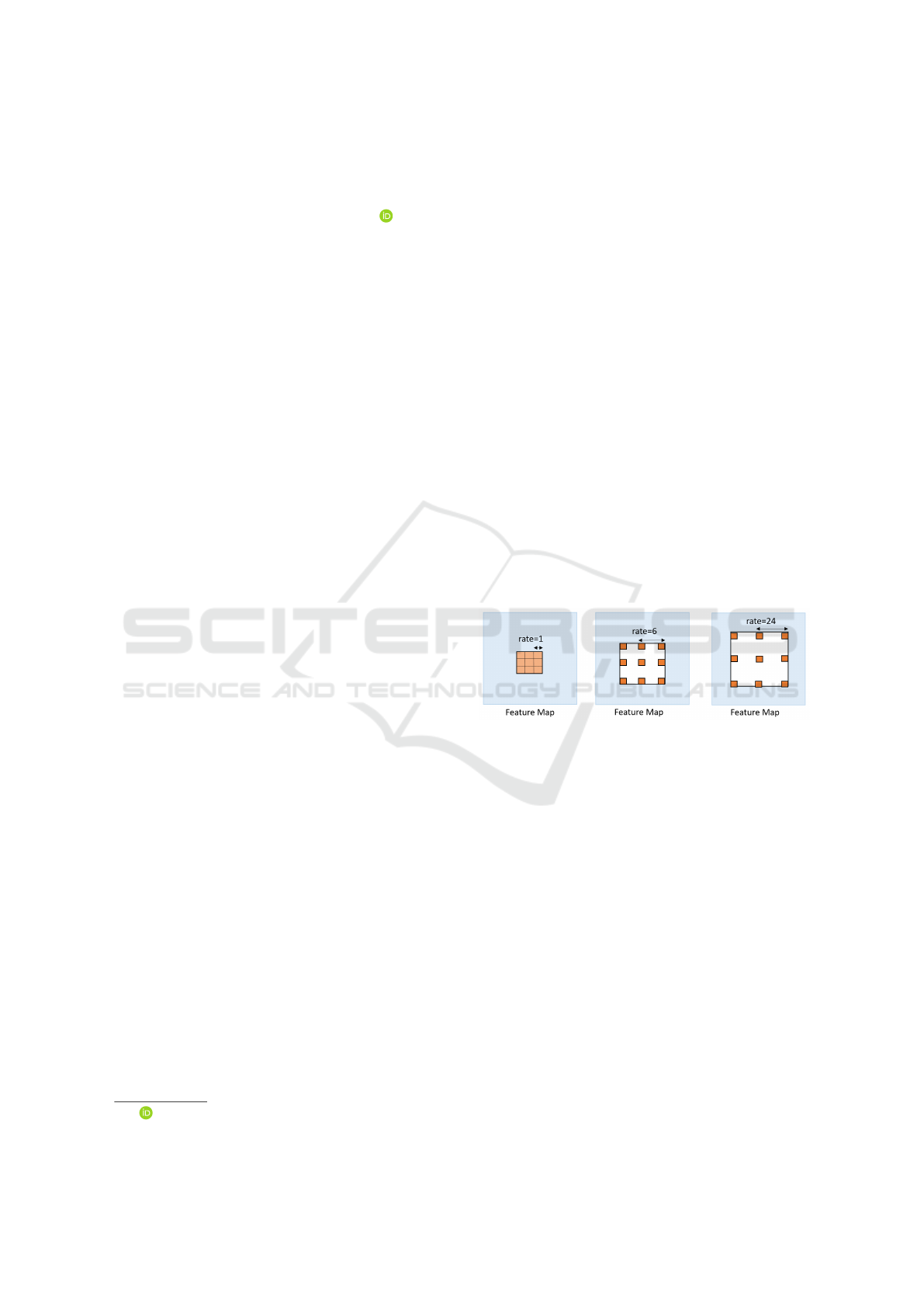
or dilation kernels have been proposed in (Fisher Yu

and Vladlen Koltun, 2016) where dilation refers to

the consideration of greater spatial resolutions of the

convolution kernels as illustrated in Fig. 1. The di-

lation rate of 1 is the standard convolution opera-

https://orcid.org/0000-0002-9374-9074

Figure 1: Dilation kernels with different dilation rates

(where rate=1 is the original convolution operation) (Chen

et al., ).

tion whereas increasing the dilation rate allows for a

larger receptive ﬁeld without increase in the number

of learnable parameters. This is achieved by adding

zeroes between the weights of the convolution kernel.

In this paper, we improve the previously proposed

dilation neural networks in two aspects. First, we re-

lax the original dilation structure for 2-dimensional

convolution which assumes equidistant sampling in

height and width of the input image. This relaxation

enables varying sampling in both input dimensions as

well as arbitrary patterns in the dilation kernels al-

lowing for a more general selection of relevant input

values (see Fig. 2). Second, this relaxation for vary-

ing sampling is made learnable through standard gra-

dient descent techniques with the variant of the log-

barrier methods for optimization. Through the pro-

posed method, we aim to solve a continuous and dis-

crete optimization problem simultaneously wherein

Chadha, G., Reimann, J. and Schwung, A.

Generalized Dilation Structures in Convolutional Neural Networks.

DOI: 10.5220/0010302800790088

In Proceedings of the 10th Inter national Conference on Pattern Recognition Applications and Methods (ICPRAM 2021), pages 79-88

ISBN: 978-989-758-486-2

the dilation parameters are encouraged to be binary

variables, in contrast to the other parameters in the

network.

The organization of the paper is as follows. Sec-

tion 2 details the related work. In section 3, the di-

lation layer together with the proposed generalized

dilation layer for CNNs is explained. Additionally,

the end-to-end training technique with the log-barrier

function along with its variants are detailed here. Ex-

perimental results on MNIST and CIFAR-10 image

datasets along with a detailed analysis of generalized

dilation layer are illustrated in section 4, with the con-

clusion detailed in section 5.

2 RELATED WORK

Convolutions with dilated ﬁlters were ﬁrst introduced

in (Holschneider et al., 1990) and (Shensa, 1992) in

the context of wavelet decomposition. Dilated convo-

lutions for deep neural networks have been initially

presented in (Fisher Yu and Vladlen Koltun, 2016)

to allow for multi-scale context aggregation without

downsampling of the resolution. Since then, dila-

tion networks have been used in semantic segmen-

tation methods due to their ability to capture large

context while preserving ﬁne details. In (L. Chen

et al., 2018), large dilation factor are used in the

Deeplab model to provide large context, which re-

sults in improved performance. This is further en-

hanced in (Chen et al., 2016) by using atrous spatial

pyramid pooling (ASPP), i.e. multi-level dilated con-

volutions, improving the results by leveraging local

and wide context information. In (Sercu and Goel,

), time dilated convolutions are used for dense pre-

diction on sequences for speech recognition, while

modeling long-distance genomic dependencies with

dilated convolutions are reported in (Gupta and Rush,

2017). Iterated dilated convolutions are applied in

(Strubell et al., 2017) for entity recognition in text

modelling for improving the performance of varia-

tional autoencoders. Dilated residual networks are in-

troduced in (Yu et al., 2017), considerably improving

vanilla residual networks (He et al., 2016) in image

classiﬁcation and segmentation. An application of di-

lation to time series analysis is provided in WaveNets

(van den Oord et al., ). However, in these works the

dilation structure is ﬁxed during training. In contrast,

we keep the dilation structure ﬂexible and end-to-end

trainable for each channel within bounds deﬁned by

the hyperparameters.

Such training of ﬂexible dilation structure has

been presented in (He et al., 2017) where a dilation

factor is trained for each channel of the convolution

layer. Furthermore, the dilation factor is deﬁned in

R instead of Z

as in the original derivation. This

comes at the cost of calculating the output map by

means of a bilinear transformation in the regular case

of fractional dilation factors. It must be noted, that

although fractional dilation factors are possible, the

structure of the dilation is still ﬁxed in this case. More

general structures are allowed by active convolutions

(Yunho Jeon and Junmo Kim, 2017), however with

low deviations from the original convolution kernel.

Deformable convolutional networks as introduced in

(Dai et al., 2017) and further improved in (Zhu et al.,

2019) allowing for similar convolution structures as

proposed by our approach. There, each point in the

convolution grid is augmented with a learnable real

valued offset. As in (He et al., 2017), a bilinear trans-

formation is needed before applying the convolution.

Contrary to the other approaches, we hold on to an up-

per limit of integer dilation factors, while allowing for

arbitrary structures of the convolution kernel within a

receptive ﬁeld using an end-to-end training method-

ology. Due to that, we end up in the exact grid po-

sition without the need for a bilinear transformation.

Finally, (Carl Lemaire et al., 2018) propose a bud-

get aware pruning methodology using the log-barrier

method. On the contrary, we propose the selection

of relevant structure in a receptive ﬁeld for efﬁcient

feature extraction.

3 GENERALIZED DILATION

NEURAL NETWORKS

In this section, we introduce generalized dilation lay-

ers starting with the description of standard dilation

networks proposed in (Fisher Yu and Vladlen Koltun,

2016).

3.1 Dilation Layer

We start with the standard discrete convolution oper-

ator deﬁned as

(F ∗ k)(p) =

∑

s+t=p

F(s) · k(t). (1)

where F and k denote the receptive ﬁeld and the con-

volution kernel respectively. In dilated convolution,

we have instead

(F ∗

k)(p) =

∑

s+lt=p

F(s) · k(t), (2)

where the term ∗

denotes the dilated convolution and

l is the dilation factor. Note that the standard convo-

lution operation is obtained for l = 1. By changing

ICPRAM 2021 - 10th International Conference on Pattern Recognition Applications and Methods

the dilation factors, the dilated convolution operator

applies the same ﬁlter (with the same parameters) at

a different range of the receptive ﬁeld and hence, al-

lows for better multiscale context aggregation (Fisher

Yu and Vladlen Koltun, 2016). The effect of the dila-

tion operation is illustrated in Figure 1 which shows

the increasing size of the ﬁlter with increasing dilation

factor.

3.2 Generalized Dilation Layers

The structure of the dilated convolution operation is

kept ﬁxed during training of a neural network. We

aim to allow for more ﬂexibility in that we want to

make the dilation structure ﬂexible and trainable. To

this end, we will ﬁrst derive an alternative representa-

tion of the dilation operation as follows. Basically, the

dilation operation can be seen as a conventional con-

volution operation with receptive ﬁeld size increased

from p × p to y × y with p < y. Correspondingly, a

larger weight matrix W ∈ R

y×y

is applied in which a

certain number of weights are ﬁxed to zero a priori

such that the active weights (weights unequal zero)

sum to p × p. Hence, we deﬁne vectors ψ

∈ {0, 1}

and ψ

∈ {0, 1}

and matrices Ψ

and Ψ

where

diag(Ψ

) = ψ

, diag(Ψ

) = ψ

. (3)

Consequently, deﬁning a new weight matrix as

W = Ψ

·W · Ψ

(4)

and using this weight matrix for convolution provides

a generalization to the dilation layer described previ-

ously. As an example, the dilation with active weight

of size 3 × 3 and dilation factor of 2 can be obtained

by deﬁning ψ

= ψ

= [1 0 1 0 1]

. Note that by arbi-

trarily setting the components of ψ

and ψ

to zero and

one while at the same time forcing the total number of

ones per ψ

and ψ

to p, arbitrary dilation structures

in the weight matrix

W can be generated. Formally,

we impose the constraints

· 1 ≤ p, ψ

· 1 ≤ p, (5)

where 1 denotes the all-one vector, yielding to ar-

bitrary dilation-like patterns. Moreover, the dilation

operation can be generalized by deﬁning a matrix

Ψ ∈ {0, 1}

y×y

and deﬁning the new weight matrix as

W = W  Ψ (6)

where  denotes element-wise multiplication. As in

the previous case, we again impose constraints on the

matrix Ψ as

Ψ · 1 ≤ p

, (7)

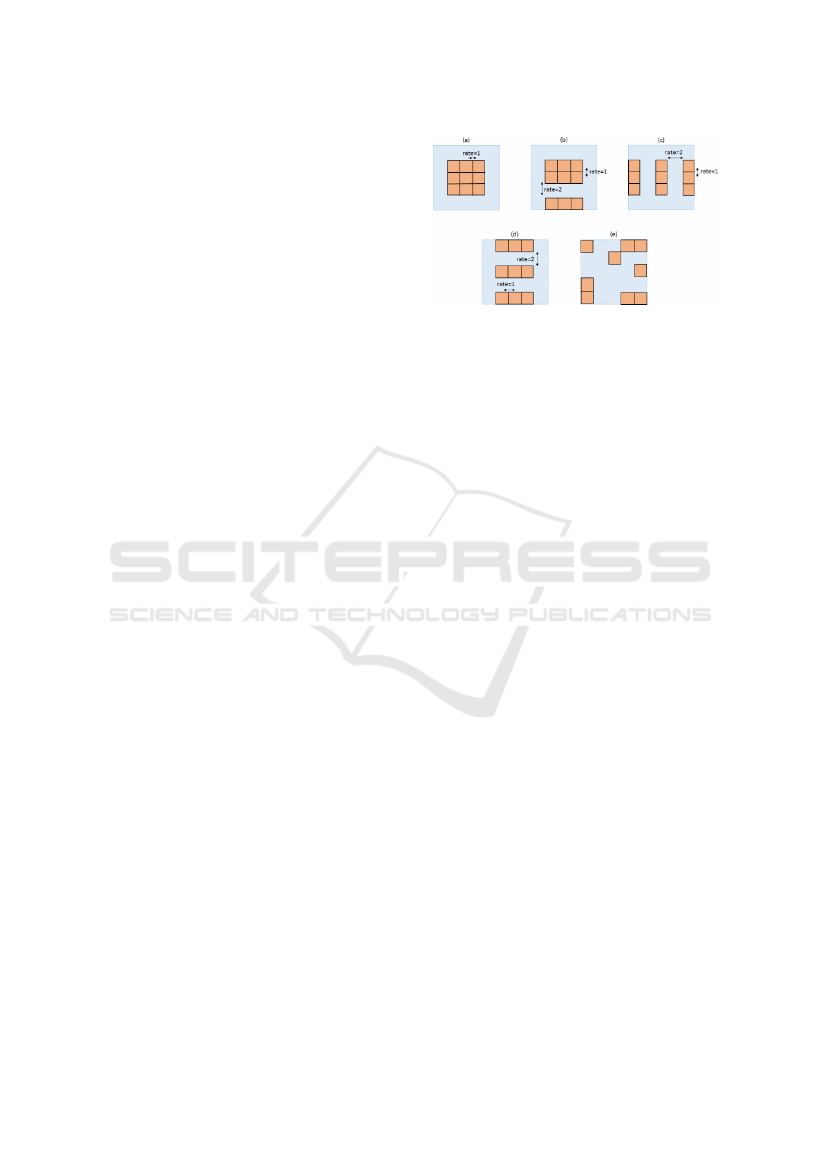
Figure 2: Different conﬁgurations of the parameters: (a)

Original convolution, (b) Dilation with varying dilation

rates; (c) Dilation in horizontal dimension only; (c) Dilation

in vertical dimension only; (e) Arbitrary dilation kernel.

which assures, that the number of weights unequal to

zero is less or equal to the kernel size. This reparam-

eterization of the weight matrix

W allows for gen-

eralized dilation structures. An illustration of some

examples for the different possible patterns is given

in Figure 2. Particularly, some choices of the pa-

rameters are useful in practice. The original convo-

lution operation (Figure 2 (a)) is obtained by setting

= ψ

= [0 1 1 1 0] while a dilation with dilation rate

2 yields ψ

= ψ

= [1 0 1 0 1]. However, this equidis-

tant choice of the dilation might not be best to obtain

representative features in some cases. This is relaxed

by setting e.g. ψ

= [0 1 1 0 1] and ψ

= [0 1 1 1 0]

resulting in non-equidistant patterns (see Figure 2 (b))

by incorporating the constraint in Eq. (5). Addition-

ally, other arbitrary dilation patterns can be realized as

shown in Figure 2 (e) by setting Ψ with the constraints

shown in Eq. (7). Higher dilation rates within the

layer can be obtained by setting p << y which results

in applying larger receptive ﬁelds. Additionally, con-

sidering multidimensional sequence modelling tasks

where longer time horizon modelling is required, di-

lation patterns as shown in Figure 2 (c) using setting

= [0 1 1 1 0] and ψ

= [1 0 1 0 1] can be beneﬁcial.

Similarly, a vertical dilation can be trained (Figure 2

(d)). Ultimately, arbitrary dilation patterns as illus-

trated in Figure 2 (e) can be obtained by setting

Ψ =







1 0 0 1 1

0 0 1 0 0

0 0 0 0 1

1 0 0 0 0

1 0 0 1 1







(8)

which is just restricted by the number of active param-

eters within the dilation kernel as presented in Eq. (7).

Higher dilation rates within the layer can be obtained

by setting p << y which results in applying larger re-

ceptive ﬁelds.

Generalized Dilation Structures in Convolutional Neural Networks

3.3 End-to-End Training of Dilation

Layers

So far we have introduced general dilation layers as

an extension of the vanilla dilation layers proposed

in (Fisher Yu and Vladlen Koltun, 2016) by deﬁning

suitable masking vectors and the relevant constraint

that is required. However, optimizing the masking

matrix and vectors results in optimizing binary vari-

ables which makes the learning problem combinator-

ical and does not directly allow for gradient based

end-to-end training. To circumvent this, we fol-

low a similar approach as in typical gating mech-

anisms (Hochreiter and Schmidhuber, 1997; Trask

et al., 2018) in that we deﬁne continuous vectors

∈ R

and matrix

Ψ ∈ R

y×y

which are passed

through a sigmoidal activation function, i.e. we de-

ﬁne

= σ(

), ψ

= σ(

), Ψ = σ(

Ψ). (9)

Using this reparameterization, the masking vector and

matrix are bounded to the interval [0, 1] and due to

the characteristics of the sigmoid function will tend to

its boundaries as training proceeds. The above repa-

rameterization helps in approximating a discrete op-

timisation problem into a continuous one. Therefore,

we end up with a trainable structure with the standard

set of network parameters ω consisting of the kernel

weights of the convolution and fully connected lay-

ers, and the proposed parameter vectors or matrices

Ψ. Since we now have a continuous approximation

of the binary variables, these can be trained by back-

propagation using off the shelf gradient descent opti-

mizers. However, we have to consider the additional

constraints on the parameters Ψ as given in Eq. (5)

and (7). These constraint have to be fulﬁlled during

training and hence, should be imposed as hard con-

straints.

In general, various approaches exist to incorpo-

rate hard constraints in stochastic gradient descent al-

gorithms, namely barrier functions, projection meth-

ods and active set methods (Boyd and Vandenberghe,

2004). In this work we propose to use barrier

functions which contribute directly to the gradients

and can approximate a hard constraint if the barrier

penalty is high enough. To this end, we include the

constraints by implementing them as a direct gradi-

ent ∇

(Ψ), based only on the layer-inherent masking

matrix Ψ of the form

∇

i j

(σ(Ψ

i j

))+b

(σ(Ψ

i j

))+b

(σ(Ψ

i j

)),

(10)

where Ψ

i j

denotes the elements of Ψ, L

denotes the

barrier loss and b

, b

and b

represents the differen-

tiable barrier function calculated over the row, column

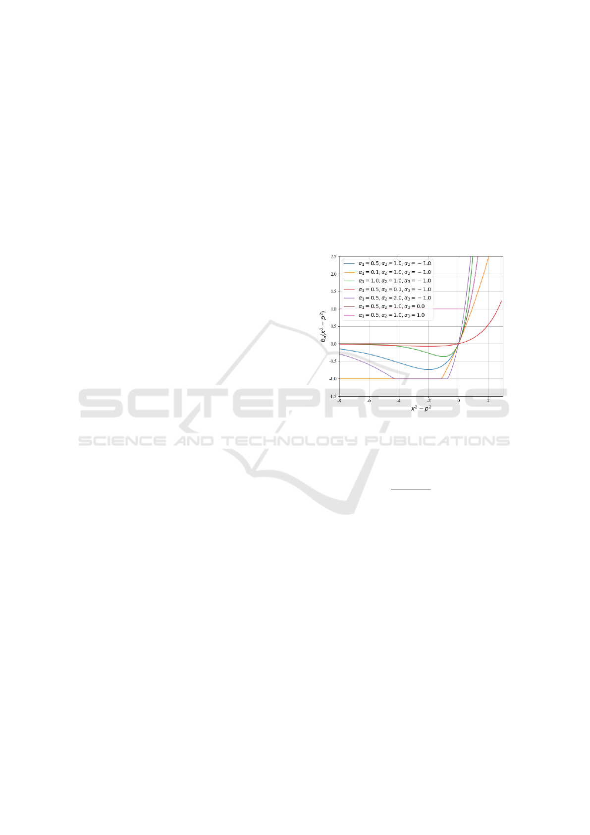
and all entries respectively. The barrier function cho-

sen is a combination of exponential and linear as in

Eq.(11) or quadratic function as in Eq.(12) where the

penalty for exceeding the constraint is higher to keep

the number of total active parameters in check.

(x)=b

(x)=max(e

·(x−p)

· α

· (x − p), α

), (11)

(x)=max(e

(

−p

)

· α



− p



, α

), (12)

Different barrier functions with the different parame-

ters α

, α

and α

are illustrated in Fig. 3. Finally,

Figure 3: Barrier functions with different parameters.

the gradient for end-to-end training of the masking

parameters yields

∇

i j

∂L

(ω, Ψ)

∂Ψ

i j

+ ∇

i j

, (13)

where L

is the classiﬁcation loss function and L

the combined loss function. We do not scale the bar-

rier loss L

with an additional hyper-parameter, and

use the barrier loss as it is. It can be useful to use

a scaled version of the barrier loss, but this can also

be accomplished with a change in one of the param-

eters α

, α

and α

. Therefore, we test with differ-

ent barrier parameters and not a regularization hyper-

parameter. Since the value of the barrier function is

used directly as the gradient for the masking parame-

ters, negative constraint values (negative in the barrier

function) result in a parameter increase, while positive

constraint values result in a parameter decrease. The

extent to which the masking parameter deviates from

its saturation depends on the both the classiﬁcation

loss L

(ω, Ψ) and barrier loss L

ICPRAM 2021 - 10th International Conference on Pattern Recognition Applications and Methods

3.4 Initialization of Masking

Parameters

The barrier functions are designed such that the gra-

dient increases exponentially if the masking matrices

are over-parameterized. Thus, the boundary condi-

tions cannot be neglected while initializing the ele-

ments in Ψ as large values of b

, b

and b

yield un-

stable gradients. Furthermore, large gradients steer

the parameter rapidly into saturating regions, which

hurts performance. This problem is solved by directly

using the information about kernel and receptive ﬁeld

size during initialization. The idea is to initialize the

masking parameters in a basin where the gradients are

not huge. Therefore, the parameters can be initialized

such that the total sigmoidal sum of all the elements

in Ψ does not exceed the constrained size of the mask-

ing matrix. Notice, that all barrier values return 0 for

σ(Ψ) = x = p, thus the elements in the masking ma-

trix are initialized by

Ψ = −ln(

− 1) ± 1. (14)

This assures, that on average, the total sum of all sig-

moidal parameters does not exceed the ﬁeld size and

thus does not break any boundary condition during

initialization, since

(

∑

1 + e

ln(

−1)

) = b

1 + e

ln(

−1)

)

(15)

= b

) = 0 (16)

and

r,c

(

∑

1 + e

ln(

−1)

) = b

r,c

(y ·

1 + e

ln(

−1)

)

(17)

= b

r,c

(

) < 0. (18)

4 EXPERIMENTS

We test the proposed generalized dilation neural net-

works (GDNN) on two different benchmark image

recognition tasks. We use the MNIST (LeCun et al.,

2010) and CIFAR-10 (Krizhevsky and Hinton, 2010)

data sets and compare the results with baseline net-

works. We analyse the effect of the different elements

in the Generalized Dilation layer and report the results

of the learnt masking and convolution ﬁlters.

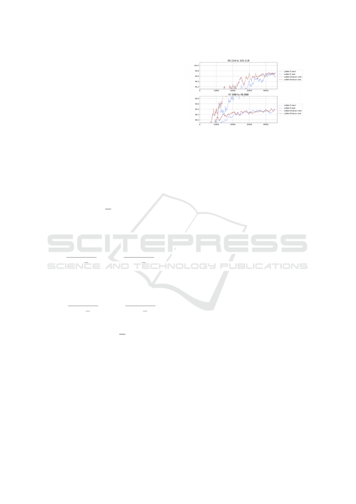
Figure 4: Accuracy graphs during training and testing over

mini-batches for LeNet and the best performing generalized

dilation network.

4.1 Experimental Results on MNIST

The initial experiments on MNIST were performed as

a sanity check for the proposed architecture. The ar-

chitecture chosen for the experiments was the same as

the LeNet (LeCun et al., 1998) architecture with the

ﬁrst convolution layer being the generalized dilation

(GD) layer with the receptive ﬁeld size of y = 9. Both

the architectures were trained for 400 epochs with a

mean test accuracy of 98.41 % and 98.43% for the

GDNN and the LeNet architecture respectively. How-

ever, the accuracy of the proposed method is consis-

tently better during training as illustrated in Fig. 4

where a zoomed in training and testing progress over

mini-batches is shown. Only during the fag end of

the training the standard LeNet architecture improves

its accuracy. After the initial test with MNIST, the

CIFAR-10 dataset was used for a more comprehen-

sive investigation.

4.2 Experimental Results on CIFAR-10

In order to analyze the performance of the GDNN

we chose the SimpleNet network (Hasanpour et al.,

2016) as a baseline architecture to investigate the

performance on the CIFAR-10 dataset. The Adam

(Kingma and Ba, 2014) optimizer with default pa-

rameters (µ = 10

−3

, β

= 0.9, β

= 0.999, ε = 10

−8

λ = 0) was used for 400 training epochs. If not stated

otherwise, we use the same experimental settings and

augmentation methods as in (Hasanpour et al., 2016).

An initial set of experiments were performed to deter-

mine the optimal location of the GD layer in the Sim-

pleNet architecture. The performance of the model

was analysed based on the performance on a held out

validation set. From this analysis, the GD layer was

found to perform best as the second (b2) and ﬁfth (b5)

layer in the SimpleNet architecture for the CIFAR-10

dataset. This points to an observation that in simple

image recognition tasks, the context aggregation fea-

Generalized Dilation Structures in Convolutional Neural Networks

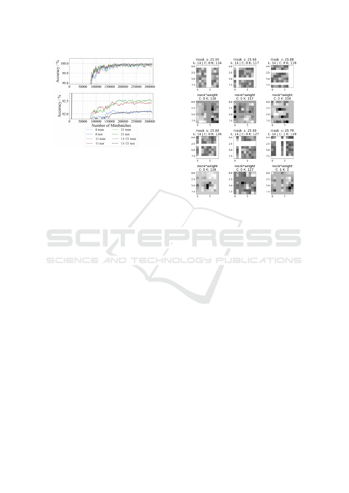
Figure 5: Training (top) and testing (bottom) accuracy

graphs for Simplenet for the two best performing general-

ized dilation networks and a combination net with 2 GD

layers.

ture of dilation kernels is useful in the earlier layers

where low level features are captured rather than the

deeper layers. Therefore, all the subsequent experi-

ments were performed with these position of the GD

layer respectively which are represented in the top and

bottom half of the Table 1. We investigate the effect

of: i. Changes in the size of receptive ﬁelds and con-

volution kernel, ii. Changes in the type of constraint

namely row, column and all constraints, iii. Changes

in the barrier function parameters namely the α, α

and α

and, and iv. Change in the number of chan-

nels of the GD layer. The ﬁnal accuracy and loss

reported in Table 1 are the best obtained values from

the network conﬁguration with the highlighted ones

being the best for the respective position of the GD

layer. Each distinct architecture tested is assigned a

number denoted in the ﬁrst column with 0 being the

vanilla SimpleNet architecture. We analyze the effect

of individual hyper-parameters which are highlighted

blue in each row. All the individual hyper-parameters

are explained in the caption of Table 1.

The foremost hyperparameter change we tested,

was the size of the receptive ﬁeld in the GD layer.

A receptive ﬁeld size of 7 performed generally bet-

ter than the its counterparts for both the GD layer

positions. Alternatively, increasing the channels for

P = 2 yielded a better test accuracy while an increase

in number of channels for P = 5 resulted in a decrease

in accuracy. This can be attributed to the bottleneck

effect where an increase in the number of output chan-

nels at the crucial bottleneck layer deteriorates perfor-

mance. A clear evidence for which type of constraint

to be used is not available since the change in perfor-

mance is not signiﬁcant enough. The effect of dif-

ferent barrier function parameters α

, α

and α

covered in the next section from the initial and learnt

Figure 6: Trained masking matrices (σ(Ψ)) and resulting

convolution kernel matrix for architecture number 3. White

pixels in the masking matrix represent σ(Ψ) = 0, while

black pixels represent σ(Ψ) = 1. Conversely, for the convo-

lution kernel matrix (σ(Ψ) · k), white and black pixels rep-

resent the corresponding minimum and maximum value for

each kernel separately. Notice, that a zero in the masking

matrix results in a constant region in the convolution matrix.

s represents

∑

, where k indicates the kernel number.

masking matrix distribution, but a stark change in the

ﬁnal performance of the network is not evident. Tests

were also performed with two GD layers in the same

network resulting in satisfactory performance but not

better than the individual networks. It is evident from

Table 1, that most permutations have a slight effect on

the ﬁnal test accuracy from the trained network. Apart

from one GDNN network, all other network outper-

form the baseline SimpleNet (denoted by Nr. 0) ar-

chitecture with a higher average test accuracy.

Figure 5 illustrates the training progress of the best

performing architectures (Architecture Number 0, 11,

21 and 11+21) for each case. The ﬁgures show a

zoomed in version to better distinguish among the ar-

chitectures. The training progress shows both GDNN

consistently and considerably outperforms the Sim-

pleNet architecture in terms of testing accuracy.

4.2.1 Dilation Kernels and Masking Parameters

A sample of the trained masking matrices and the ef-

fective convolution ﬁlters are shown in Fig. 6 as grey-

scale maps where the headings on each of the masking

maps represent the sum of all the sigmoidal parame-

ICPRAM 2021 - 10th International Conference on Pattern Recognition Applications and Methods

Table 1: Different permutations of network architectures and their ﬁnal training and testing results. Highlighted entries

represent hyperparameters deviating from the baseline nets and the highest accuracy or lowest loss respectively. Exp. Nr.=

Distinct Architecture Number, P = Position of Generalized Dilation layer, L = Number of GD Layers, C = Number of GD

channels, p = Convolution kernel size, F = Size of Receptive Field, Constraints are deﬁned as r = only rows, c = only columns

and a = all.

Arch. Nr. P L C p F α

Constraints Train Test

Loss Acc. Loss Acc.

·10

−2

% ·10

−2

0 2 - 128 3 - - - - - 0.042 99.98 66.64 91.99

b2 2 1 128 3 7 0.5 1 -1 r,c,a 0.040 99.98 64.74 92.32

1 2 1 128 3 9 0.5 1 -1 r,c,a 0.048 100.0 68.47 91.82

2 2 1 128 5 7 0.5 1 -1 r,c,a 0.088 99.97 66.62 92.38

3 2 1 128 5 9 0.5 1 -1 r,c,a 0.010 100.0 67.84 91.53

4 2 1 128 3 7 0.5 1 -1 r,c 0.045 99.84 61.79 92.15

5 2 1 128 3 7 0.5 1 -1 r 0.053 99.98 64.02 92.23

6 2 1 128 3 7 0.5 1 -1 a 0.068 99.97 64.78 92.15

7 2 1 128 3 7 0.1 1 -1 r,c,a 0.015 100.0 64.67 92.22

8 2 1 128 3 7 0.5 0.1 -1 r,c,a 0.068 99.98 67.06 92.00

9 2 1 128 3 7 0.5 1 0 r, c, a 0.056 99.98 67.37 92.01

10 2 1 64 3 7 0.5 1 -1 r,c,a 0.086 99.97 66.95 91.58

11 2 1 256 3 7 0.5 1 -1 r,c,a 0.018 100.0 66.09 92.48

b5 5 1 256 3 7 0.5 1 -1 r,c,a 0.055 99.97 62.64 91.94

12 5 1 256 3 9 0.5 1 -1 r,c,a 0.026 99.98 62.64 91.56

13 5 1 256 5 7 0.5 1 -1 r,c,a 0.019 100.0 62.28 91.84

14 5 1 256 5 9 0.5 1 -1 r,c,a 0.038 99.97 62.31 92.08

15 5 1 256 3 7 0.5 1 -1 r,c 0.169 99.97 62.47 92.17

16 5 1 256 3 7 0.5 1 -1 r 0.055 99.98 62.91 92.15

17 5 1 256 3 7 0.5 1 -1 a 0.008 100.0 59.03 92.13

18 5 1 256 3 7 0.1 1 -1 r,c,a 0.049 99.98 60.61 91.91

19 5 1 256 3 7 0.5 0.1 -1 r,c,a 0.042 99.98 58.62 92.23

20 5 1 256 3 7 0.5 1 0 r, c, a 0.007 100.0 59.18 92.20

21 5 1 128 3 7 0.5 1 -1 r,c,a 0.206 99.92 59.69 92.44

22 5 1 512 3 7 0.5 1 -1 r,c,a 0.065 99.97 62.99 91.96

11+21 2,5 1,1 128,256 3 7 0.5 1 -1 r,c,a 0.024 99.98 64.19 92.08

ters, layer number, channel number and kernel num-

ber. It is evident here that the optimizer separates out

speciﬁc columns and rows, based on the constraints

i.e. the difference between the receptive ﬁeld size and

the kernel size is big enough. From Fig. 6, a gen-

eralized dilation kernel is clear where only the most

useful parts from the receptive ﬁelds are considered

for training the network. This behaviour can be sup-

pressed or emphasized depending on the α and other

barrier parameters. For similar sizes between recep-

tive ﬁelds and kernel size, the ﬁnal masking matrices

tend to be the same value for each entry, since the

constraints are not forcing enough.

To better visualise the training of the proposed

masking matrices, a distribution plot of the initial

and learned masking parameters for solitary GD layer

networks, speciﬁcally architecture number 11 and 21

(top and middle) and a network with two GD layers

(bottom) is shown in Figure 7.The initialization was

consistent in all the cases because of the initialization

methodology of Ψ mentioned in Eq. (14). Surpris-

ingly, the layers of the network with two GD layers

are trained to almost the same distribution. This can

be attributed to the speciﬁc conﬁguration of barrier

functions where the learned distribution seems to be

the optimal distribution. In the case of two GD layer

network, the barrier function from the last generalized

dilation layer do not have a direct impact on the gra-

dients backpropagated to the previous layers, but the

varying output of the ﬁrst generalized dilation layer

should result in a different input images for the lat-

ter layers. The fact that the distributions are still the

same can only be interpreted as an optimal solution

for these chosen hyperparameters.

Changing the barrier function hyperparameter α

results in a small but noticeable difference in clas-

siﬁcation accuracy, but the masking distributions

change drastically. The masking distributions from

Generalized Dilation Structures in Convolutional Neural Networks

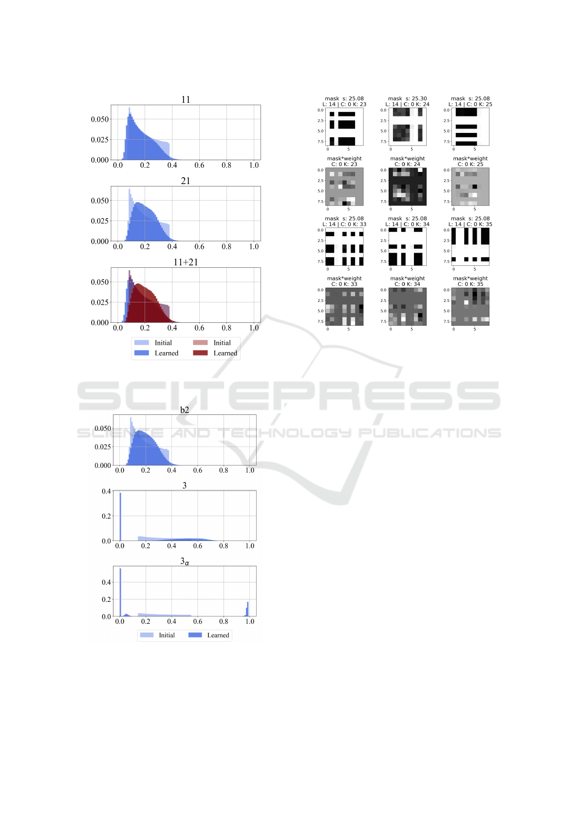
Figure 7: Distribution of masking parameters σ(Ψ) for ar-

chitecture number 11 (top) , 21 (middle) and 11 + 21 (bot-

tom).

Figure 8: Distribution of masking parameters σ(Ψ) for the

architecture number b2 (top), 3 (middle) and 3

(bottom).

Figure 9: Trained masking matrices (σ(Ψ)) and resulting

convolution matrix for architecture number 3. White pix-

els in the masking matrix represent σ(Ψ) = 0, while black

pixels represent σ(Ψ) = 1. For the convolution matrix

(σ(Ψ) · k), white and black pixels represent the correspond-

ing minimum and maximum for each kernel separately. No-

tice, that a zero in the masking matrix results in a constant

region in the convolution matrix. s represents

∑

σ(Ψ

whereas k indicates the kernel number.

architecutre numbers b2, 3 and 3 with an additional

increase in α

, from hereon called 3

, are shown in

Figure 8. Network b2 has a very similar masking

distribution compared to 11, 21 and 11 + 21 since

all parameters regarding the constraint function are

the same, they only differ in the convolution kernel

and receptive ﬁeld size. However, the networks 3

and 3

show a very different distribution of mask-

ing parameters: σ(Ψ) tends to be close to zero or

one in most cases, pointing to a binary learnt mask-

ings that have converged in choosing speciﬁc pixels

completely and ignoring other pixel values. This be-

haviour is also visible in Figure 9 wherein the masks

from architecture 3 have blocked out certain areas of

the feautre maps that are not relevant for the classiﬁ-

cation task. Therefore, with an appropriate choice of

the barrier function parameters, a continuous approx-

imation for a discrete optimization problem has been

demonstrated.

ICPRAM 2021 - 10th International Conference on Pattern Recognition Applications and Methods

5 CONCLUSION

We present generalized dilation neural networks, a

sub-module within the CNN architecture augmented

with dilated ﬁlters. The generalization to the exist-

ing framework is provided by two extensions. First,

the ﬁxed dilation ﬁlters are made learnable by intro-

ducing an alternative continuous representation of the

dilation operation using masking vectors or matrices

which can be trained by standard gradient descent op-

timizers. To this end, we introduce a novel barrier

function approach together with a suitable initializa-

tion scheme to account for the constraints imposed

on the masking parameters. According to the au-

thors, this is the ﬁrst study which makes use of such

techniques for constraining the dilation operation in a

CNN. Second, we generalize the ﬁxed structure of di-

lation kernels to arbitrary structures, allowing for an

arbitrary coverage of the input space. We provide ex-

perimental evidence by testing the proposed architec-

ture on two benchmark image recognition data-sets.

The learned masking maps and distributions point to

a discrete optimization of parameters using continu-

ous gradient descent methods.

Although not presented in the results, the gener-

alized dilations can also be applied on the whole in-

put image rather than a receptive ﬁeld, leading to a

form of barrier function based attention. Using this

architecture as the very ﬁrst layer of a CNN with an

receptive ﬁeld size equal to the input size, the layer

is forced to select only certain discriminative pixels

from the actual input. Also part of the future work is

the use of barrier function for selecting a certain num-

ber of channels in the convolution layers where com-

plete channels will be masked out from training lead-

ing to a sparse network. On the application side, we

will experiment with GDNN on domains like image

segmentation, object detection and sequential mod-

elling. Such tasks are suitable as the networks need

to produce even denser predictions, for e.g. a predic-

tion for each pixel.

REFERENCES

Bai, S., Kolter, J. Z., and Koltun, V. (2018). An em-

pirical evaluation of generic convolutional and recur-

rent networks for sequence modeling. arXiv preprint

arXiv:1803.01271.

Boyd, S. P. and Vandenberghe, L. (2004). Convex optimiza-

tion. Cambridge University Press, Cambridge.

Carl Lemaire, Andrew Achkar, and Pierre-Marc Jodoin

(2018). Structured pruning of neural networks with

budget-aware regularization. 2019 IEEE/CVF Con-

ference on Computer Vision and Pattern Recognition

(CVPR), pages 9100–9108.

Chen, L.-C., Papandreou, G., Schroff, F., and Adam, H. Re-

thinking atrous convolution for semantic image seg-

mentation.

Chen, L.-C., Yang, Y., Wang, J., Xu, W., and Yuille, A. L.

(2016). Attention to scale: Scale-aware semantic im-

age segmentation. In Proceedings of the IEEE con-

ference on computer vision and pattern recognition,

pages 3640–3649.

Dai, J., Qi, H., Xiong, Y., Li, Y., Zhang, G., Hu, H., and

Wei, Y. (2017). Deformable convolutional networks.

In Proceedings of the IEEE international conference

on computer vision, pages 764–773.

Fisher Yu and Vladlen Koltun (2016). Multi-scale context

aggregation by dilated convolutions. In ICLR.

Fukushima, K. and Miyake, S. (1982). Neocognitron: A

self-organizing neural network model for a mecha-

nism of visual pattern recognition. In Competition and

cooperation in neural nets, pages 267–285. Springer.

Gupta, A. and Rush, A. M. (2017). Dilated convolu-

tions for modeling long-distance genomic dependen-

cies. bioRxiv.

Hasanpour, S. H., Rouhani, M., Fayyaz, M., and Sabokrou,

M. (2016). Lets keep it simple, using simple architec-

tures to outperform deeper and more complex archi-

tectures. arXiv preprint arXiv:1608.06037.

He, K., Zhang, X., Ren, S., and Sun, J. (2016). Deep resid-

ual learning for image recognition. In Proceedings of

the IEEE conference on computer vision and pattern

recognition, pages 770–778.

He, Y., Keuper, M., Schiele, B., and Fritz, M. (2017).

Learning dilation factors for semantic segmentation

of street scenes. In German Conference on Pattern

Recognition, pages 41–51.

Hochreiter, S. and Schmidhuber, J. (1997). Long short-term

memory. Neural computation, 9(8):1735–1780.

Holschneider, M., Kronland-Martinet, R., Morlet, J., and

Tchamitchian, P. (1990). A real-time algorithm for

signal analysis with the help of the wavelet transform.

In Wavelets, pages 286–297. Springer.

Kingma, D. P. and Ba, J. L. (2014). Adam: Amethod for

stochastic optimization. In Proceedings of the 3rd In-

ternational Conference on Learning Representations

(ICLR).

Krizhevsky, A. and Hinton, G. (2010). Convolutional deep

belief networks on cifar-10. Unpublished manuscript,

40(7).

L. Chen, G. Papandreou, I. Kokkinos, K. Murphy, and A. L.

Yuille (2018). Deeplab: Semantic image segmentation

with deep convolutional nets, atrous convolution, and

fully connected crfs. IEEE Transactions on Pattern

Analysis and Machine Intelligence, 40(4):834–848.

LeCun, Y., Boser, B. E., Denker, J. S., Henderson, D.,

Howard, R. E., Hubbard, W. E., and Jackel, L. D.

(1990). Handwritten digit recognition with a back-

propagation network. In Advances in neural informa-

tion processing systems, pages 396–404.

Generalized Dilation Structures in Convolutional Neural Networks

LeCun, Y., Bottou, L., Bengio, Y., and Haffner, P. (1998).

Gradient-based learning applied to document recogni-

tion. Proceedings of the IEEE, 86(11):2278–2324.

LeCun, Y., Cortes, C., and Burges, C. J. (2010). MNIST

handwritten digit database. AT&T Labs [Online].

Available: http://yann. lecun. com/exdb/mnist, 2.

Luo, W., Li, Y., Urtasun, R., and Zemel, R. (2016). Under-

standing the effective receptive ﬁeld in deep convolu-

tional neural networks. In D. D. Lee, M. Sugiyama,

U. V. Luxburg, I. Guyon, and R. Garnett, editors, Ad-

vances in Neural Information Processing Systems 29,

pages 4898–4906. Curran Associates, Inc.

Sercu, T. and Goel, V. Dense prediction on sequences with

time-dilated convolutions for speech recognition.

Shensa, M. J. (1992). The discrete wavelet transform: wed-

ding the a trous and mallat algorithms. IEEE Transac-

tions on Signal Processing, 40(10):2464–2482.

Strubell, E., Verga, P., Belanger, D., and McCallum, A.

(2017). Fast and accurate entity recognition with iter-

ated dilated convolutions. In Proceedings of the 2017

Conference on Empirical Methods in Natural Lan-

guage Processing, pages 2670–2680, Copenhagen,

Denmark. Association for Computational Linguistics.

Trask, A., Hill, F., Reed, S. E., Rae, J., Dyer, C., and Blun-

som, P. (2018). Neural arithmetic logic units. In

Advances in Neural Information Processing Systems,

pages 8035–8044.

van den Oord, A., Dieleman, S., Zen, H., Simonyan, K.,

Vinyals, O., Graves, A., Kalchbrenner, N., Senior, A.,

and Kavukcuoglu, K. Wavenet: A generative model

for raw audio.

Yu, F., Koltun, V., and Funkhouser, T. (2017). Dilated

residual networks. In Proceedings of the IEEE con-

ference on computer vision and pattern recognition,

pages 472–480.

Yunho Jeon and Junmo Kim (2017). Active convolution:

Learning the shape of convolution for image classiﬁ-

cation. 2017 IEEE Conference on Computer Vision

and Pattern Recognition (CVPR), pages 1846–1854.

Zhu, X., Hu, H., Lin, S., and Dai, J. (2019). Deformable

convnets v2: More deformable, better results. In Pro-

ceedings of the IEEE Conference on Computer Vision

and Pattern Recognition, pages 9308–9316.

ICPRAM 2021 - 10th International Conference on Pattern Recognition Applications and Methods