
Applying Automated Machine Learning to Improve Budget
Estimates for a Naval Fleet Maintenance Facility
Cheryl Eisler
1
and Mikayla Holmes
2
1
Centre for Operational Research and Analysis, Defence R&D Canada, 60 Moodie Drive, Ottawa, Canada
2
University of Victoria, Department of Mathematics and Statistics, 3800 Finnerty Road (Ring Road), Victoria, Canada
Keywords: Automated Machine Learning, Predictive Analytics, Budget, Overtime Hours, Fleet Maintenance Facilities,
Work Orders.
Abstract: A study was undertaken to improve the accuracy of staffing overtime budget predictions for a naval fleet
maintenance facility and identify primary factors associated with overtime accrual. A series of models based
on facility work orders were developed using the R statistical suite and the open source package H2O.ai for
automated machine learning. Along with the model's predictive capabilities for budgetary planning, primary
work order attributes associated with overtime hours were also determined based on the variables of
importance. These gave insight into the type of maintenance and personnel assigned to the maintenance task
which contributed to the highest accrual of overtime hours. Additionally, the monthly best curve fit for past
budget predictions revealed a sigmoidal relationship, which was used to assist in the prediction of fiscal year
2019/2020 budget. The budget estimate from the model was found to be within 5% of the total budget
expended hours over the fiscal year. As new annual data are provided or additional facilities examined, the
models can be retrained or rebuilt to include new information and allow decision makers to prepare more
accurate funding estimates – potentially reserving funds for upcoming critical maintenance tasks or saving
funds through alternative approaches to task management.
1 INTRODUCTION
The Royal Canadian Navy (RCN) maintains its fleet
of warships, submarines and other auxiliary
formation vessels using a combination of internal and
external services. First-line maintenance addresses
immediate, limited repairs and minor functionality
issues on-board the ships. Second-line work includes
corrective maintenance conducted at a repair facility,
such as fixing seals or replacing bearings. The most
common third-line work, known as repair and
overhaul, involves repairing both damaged and worn
vessel components, as well as component
replacement at end of service life. Second- and third-
line maintenance may be conducted internally at a
Fleet Maintenance Facility (FMF) or externally
through an in-service support contract. The RCN
operates two such facilities, each collocated with a
naval base.
Within these RCN facilities, maintenance tasks
are broken down into Work Orders (WOs); where
each WO is documented to capture: (1) the type of
work to be completed; (2) client organization; (3) the
platform on which the work is to be completed; and
(4) a variety of other characteristics pertaining to the
task. It may be necessary to approve the use of
overtime (OT) to close WOs, as necessitated by
operational requirements. The need for OT is
dependent on the operational impact and urgency of
the task, the current workload, and the authorized OT
budget. Thus, a study was undertaken to improve the
accuracy of FMF overtime budget predictions and
identify primary factors associated with OT accrual
(Holmes, 2020). One FMF supplied seven years of
past OT data, budgets, and WO attributes to facilitate
trend analysis and to identify major variables of
importance for OT accrual.
A literature review was conducted to determine
similar classes of problems and identify an
appropriate methodology to predict both total OT for
a given WO and month within the Fiscal Year (FY)
that the OT is accrued based on the attributes of the
WO. Based on this review and its operational
capabilities, an Automated Machine Learning
(autoML) approach using H2O was deemed the most
applicable to the study. The results of this survey are
586
Eisler, C. and Holmes, M.
Applying Automated Machine Learning to Improve Budget Estimates for a Naval Fleet Maintenance Facility.
DOI: 10.5220/0010302205860593
In Proceedings of the 10th International Conference on Pattern Recognition Applications and Methods (ICPRAM 2021), pages 586-593
ISBN: 978-989-758-486-2
Copyright
c
2021 by SCITEPRESS – Science and Technology Publications, Lda. All rights reserved

presented in Section 2. Utilizing the common pipeline
process for autoML described by Truong et al.
(2019), the analysis is broken down into data pre-
processing, feature engineering, model generation,
and model interpretation. In Section 3.1 and 3.2, past
data regarding OT and WOs were processed to
establish trends, identify correlations, and develop
features. Explained in Section 3.3, an autoML
predictive model was developed. Section 3.4
illustrates how the model is used to estimate the FY
2019/2020 (FY19/20) OT budget with a target of
±5% accuracy. Future work to improve the model
accuracy is outlined in Section 4. Conclusions
presented in Section 5.
2 LITERATURE REVIEW
FMFs process hundreds of thousands of WOs every
year, only a portion of which require overtime to
complete. Overtime hours are accrued by personnel
completing specific types of maintenance tasks,
driven by a number of factors such as operational
demand tempo for ready naval vessels, number, age
and types of vessels in fleet, maintenance policies,
supply chain logistics or tool availability constraints,
resource limitations, or human resource policies.
A similar Canadian defence application using
supervised machine learning algorithms (Maybury,
2018) – specifically classification and regression
trees – examined the variables of importance
associated with maintenance task completion times.
WO were clustered based on completion times to
determine the attributes which influenced length of
time necessary for specific tasks. Finding such
variables of importance is but one aspect of the study
described herein. Further insights were obtained on
data cleaning, as well as analysing and manipulating
the data in the R statistical suite. This was valuable
for data pre-processing.
The predictive powers of Random Forests (RF),
Gradient Boosted Machines (GBM), support vector
machines and general linear models were presented
by Ellis et al. (2015) to predict wind power variability
based on occurrence of extreme wind events of wind
farms in Southern Australia. After comparing
predictive power, reliability, and tuning ease, results
indicated that RF and GBM generated reliable
models. These techniques could be leveraged to gain
insight to the general trends and correlations present
in the WO datasets. As these models are also often
used in automated machine learning, understanding
their application and use also aids in interpreting the
output from autoML tools.
Likewise relevant for the predictive outcomes of
analysis, (Bartek et al., 2018) sought to optimize
operating room usage by improving estimations of
case-time duration to reduce the number of cases that
exceed 10% of the estimated operating time.
Estimates of case-time duration in operating rooms
was optimized using extreme gradient boosting,
which is a variation of the gradient boosting
algorithm (Friedman, 2001). The way machine
learning models were used to improve upon
efficiency in scheduling and cost savings in Bartek et
al. (2018) was emulated for the study herein to
determine primary factors associated with OT for
WOs. Such identification of variables of importance
provided the foundation for feature engineering prior
to model generation.
Tools for automating the machine learning
pipeline from end-to-end to reduce the time and effort
spent on repetitive tasks were explored. A variety of
open source tools are available for use, and have been
compared in the literature (Balaji, Allen, 2018;
Gijsbers et al., 2019; He et al., 2020; Truong et al.,
2019). Overall, H2O autoML is able to handle all
input data types, performs well in a per model
classification comparison, is open source, and is easy
to use.
Notably, a tool such as H2O autoML predicts on
a single output variable of interest. This informed the
approach, as there were two variables to predict here:
the amount of OT hours (a non-negative numeric
value) and month OT accrued by WO (categorical).
This combination of predictors puts the problem in a
restricted subset of similar estimation tasks – where
the accrual of OT hours is a combination of a failure
prediction/detection and dynamic costing, and the
month of accrual is time dependent. While many
machine learning applications predict a single (and
often binary) variable using time series (e.g., Gohel et
al. (2020)), few attempt a combined variable model
approach (Baykasoğlu et al., 2009; Desai et al., 2020;
Ganapathi et al., 2009; Guanoluisa, 2020; Naik et al.,
2019; Ozturk, Fthenakis, 2020).
3 ENGAGING THE AUTOML
PIPELINE
To build a thorough understanding of the variables of
importance for OT accrual, identify correlations
between WO variables, and establish appropriate
datasets on which to predict the output variables, it
was necessary to engage a human-in-the-loop during
the data pre-processing and feature engineering
Applying Automated Machine Learning to Improve Budget Estimates for a Naval Fleet Maintenance Facility
587
phases of the autoML pipeline. This enabled two
separate models to be generated, followed by
automatic hyperparameter optimization and
architecture search. The final model interpretation
was crossed checked against previous models, and the
predictive analysis visualized.
3.1 Data Pre-processing
To prepare the data for exploration, the data
collection, cleaning and augmentation steps were
performed with significant oversight and human
intervention to ensure that a solid understanding of
the problem was obtained at the start of the process.
3.1.1 Data Collection
Datasets were limited to the past seven years
(FY13/14-FY19/20) of information extracted from
official records management systems. To predict for
two variables of output, it was necessary to have two
separate, although linked, datasets from which to
build each model. Thus, to determine the amount of
OT accrued, a dataset with all past WOs from
FY13/14-FY18/19 (for model development, referred
to as Dataset A) was used. A snapshot of the open WO
near the beginning of FY19/20 was collected for
predictive purposes (Dataset A
p
). These data detailed
information associated work order identification (ID),
history, maintenance specifics, and financial coding.
The second dataset was only those WO that
accrued OT (referred to as Dataset B). These data
detailed information associated with work order
identification, overtime hours by date, and
classification of personnel assigned. Both datasets
included numerical, categorical and time-series data.
3.1.2 Data Cleaning
Datasets included numerical (e.g., WO ID, OT
Hours), categorical (e.g., Activity Type, Work
Centre) and time-series data (Date of OT Hour
Accrual). In many cases, the categorical fields were
based on free-form text that either had to be cleaned
to fit a set of consistent categories or built from a
common understanding of key words in the text.
3.1.3 Data Augmentation
New data was created in the datasets by splitting free-
form text fields into multiple categories. In some
cases, numerical codes were aligned with text
categories to link columns together, easing human
interpretability.
3.2 Feature Engineering
A variety of tools were utilized to transform the raw
data into features that better represent the underlying
problem. These ranged from simple regression
analysis to use of RFs and GBMs. To understand WO
attributes that influenced the accrual of OT, data was
organized by FY based on total OT accrued.
3.2.1 Feature Selection
It was important to discern whether trends between
FYs had large variability prior to deciding which FYs
were suitable to build final datasets for predictive
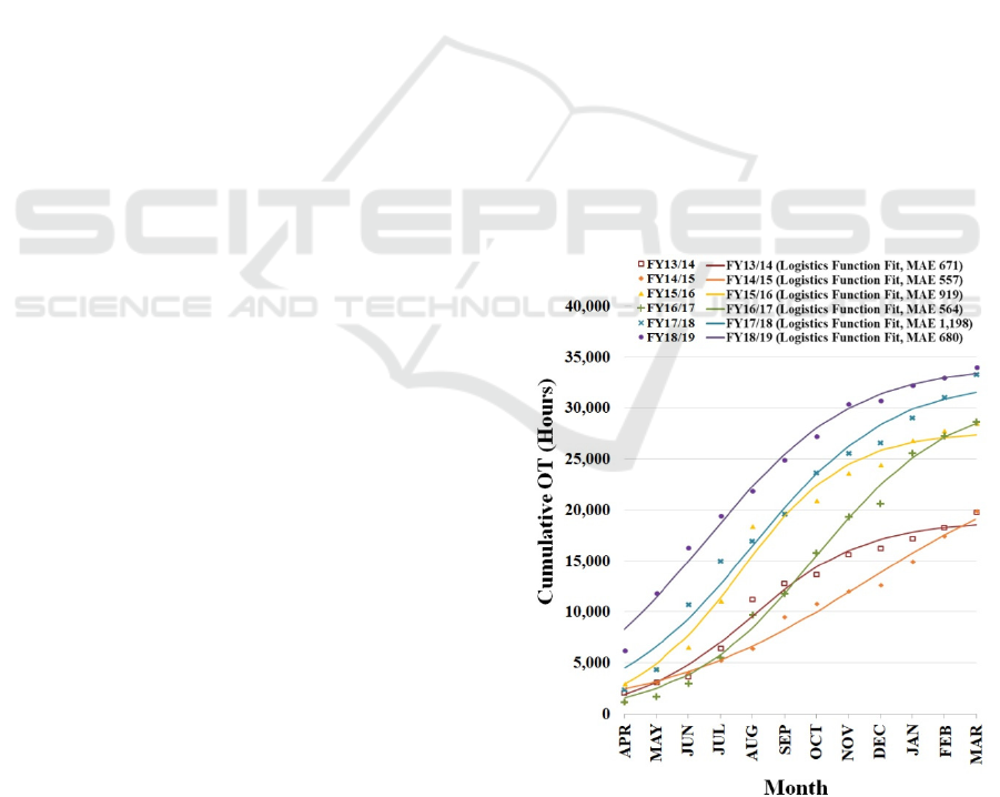
modelling (Ebadi et al., 2019). First, the OT hours
accrued by month, for each FY was plotted and curve
fits were obtained to better establish the relationship
between time and total accrual. Figure 1 illustrates
cumulative OT has a sigmoidal shape with the mean
average error (MAE) for a logistics function best fit
of 2.8% of total hours with a standard deviation of
±0.64%. Residual plots for each fit (not shown here)
were analysed and confirmed the logistics function fit
(Kassambara, 2018). Logistics functions can
logically be expected in situations where budgets are
not immediately known at the start of the FY, the
busiest seasons align with the middle of the FY, and
budget caps spending near the end of the FY.
Figure 1: Cumulative OT accrual from FY13/14 to FY18/19
with logistics function fit.
ICPRAM 2021 - 10th International Conference on Pattern Recognition Applications and Methods
588
When examining features, Non-Billable work was
the second highest contributor of OT each FY, except
in FY 13/14 where it contributed the most OT hours.
Although FY 13/14 and FY 14/15 were
observably distinct from latter FYs in the fewer
amount of OT accrued and who accrued OT, it was
decided that FY 13/14 and FY 14/15 must be initially
retained to assist training of the machine learning
algorithm. Ideally, these earliest FYs will eventually
be removed from the model building process once
more recent data is obtained.
3.2.2 Feature Construction and Extraction
To build a model which used all available FYs as
training data, Datasets A and B were stacked. To
address potential issues in the use of autoML
techniques, checks for multicollinearity and
correlation of dataset fields were completed (Ebadi et
al., 2019). A regression model that contains severe
multicollinearity between variables can cause the
coefficients of those variables to have high standard
errors, resulting in instability when presented with
new data. Multicollinearity and correlation can also
cause the importance of those variables to be skewed
or masked, resulting in a model which can be difficult
to interpret, especially if the correlated variables are
ones of interest (Allison, 2012).
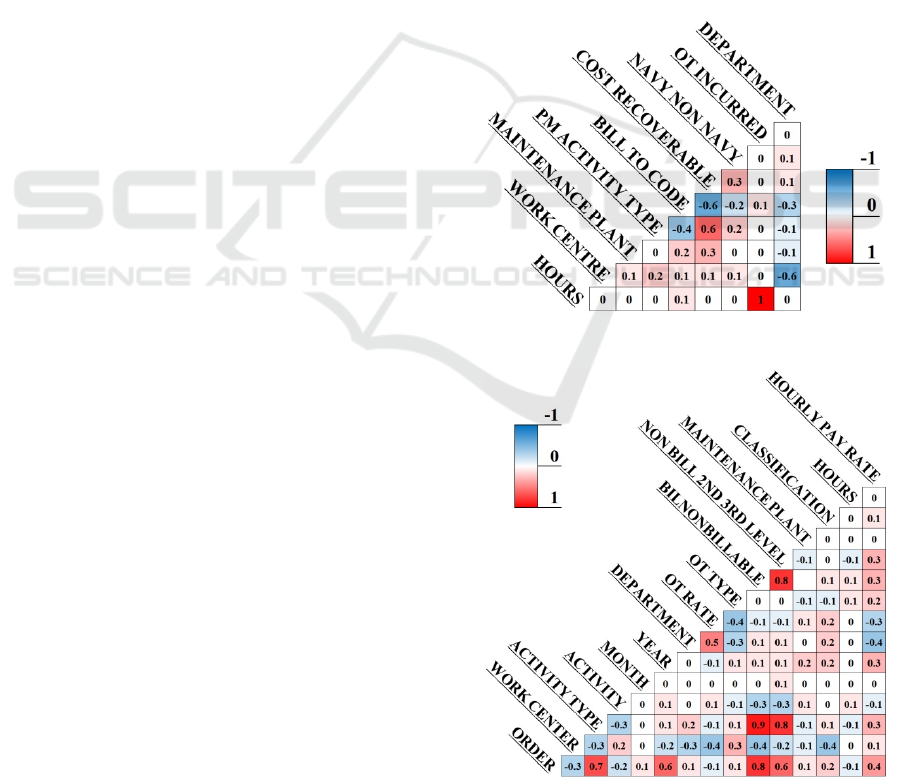
Shown in Figure 2 is a sample correlation graph
demonstrating strong correlation of variables from
Dataset A, with darker shades of blue or red
corresponding to the strength of negative or positive
correlation, respectively. Figure 3 illustrates the
correlation graph for Dataset B.
Algorithms that are efficient at predicting a
continuous variable with only categorical variables as
predictors were examined, as well as unbalanced
datasets like the ones used for this study. Unbalanced
datasets are those which consist of one outcome being
substantially more frequent than others. For this
analysis, the average number of WO which incur OT
is 3.8% each FY, thus > 96% of WOs should be
predicted to return zero OT hours per WO.
Also, given the high number of categories (over
100) within the data columns, it was desired to find
algorithms which performed well without the need for
encoding and could have dependent input variables.
As such, tree-based models were pursued.
Tree-based models can handle correlation
between predictor variables effectively because they
only consider variables that improve the error
function at each local split, inherently ignoring one of
each pair of correlated variables. To interpret models
which have multicollinearity, best practice is to build
models with one of the correlated variables removed
to determine how its presence affects relative
importance calculations (Ebadi et al., 2019).
Initial models were built using simple decision
and regression trees, as they provided initial insight
by displaying variables of importance. For example
in Dataset A, predicting the fields for Hours per WO
using decision and regression trees (Therneau et al.,
2017), Bill-To Code was found to be a significant
variable of importance. This is expected, as Figure 2
shows that Bill-To Code was (positively or
negatively) correlated with PM Activity Type, Cost
Recoverable and Department. To unmask the
importance of these variables, Bill-To Code was not
subsequently used as an input. Furthermore, the Cost
Recoverable field had little impact on the variables of
importance and was not used subsequently to increase
the accuracy of the PM Activity Type (Holmes,
2020).
Figure 2: Correlation graph for Dataset A (all WOs).
Figure 3: Correlation graph for Dataset B (only those WOs
with accrued OT).
Applying Automated Machine Learning to Improve Budget Estimates for a Naval Fleet Maintenance Facility
589
Differences in variables of importance were
examined further with RF and GBM algorithms to
determine if data from all FYs could be combined to
obtain one large dataset to build a final model. As the
standard packages in R were limited to categorical
input variables with 52 levels or less, a new package
for analysis was sought.
H2O is an open source package available for R (as
well as other languages) that is proficient at handling
big data, and is also user-friendly. It facilitates the
building, training and testing of a variety of machine
learning models (H2O.ai, 2020). For the remainder of
the analysis, all models discussed were built using
H2O’s algorithms.
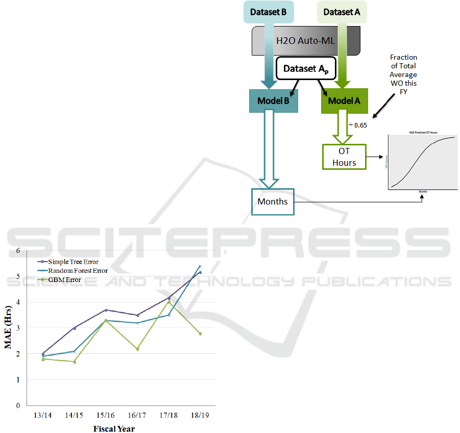
Both RF and GBM models were created and the
error on the results for all models were compared in
Figure 4. To compare each models prediction
accuracy, the MAE metric from the validation data
was used throughout. Seeing improvement in both the
average MAE, as well as steadier variables of
importance, indicated that trends were deemed to be
similar enough across fiscal years to justify building
a stacked dataset. Ideally, the years which showed
discrepancies would be removed; however, the need
for a larger training dataset was greater initially, and
therefore all years will be kept in until further data is
obtained.
Figure 4: MAE between predicted and actual OT Hours per
WO from Dataset A for all feature extraction models.
3.3 Model Generation
Next, H2O autoML was used to build two models, as
shown in Figure 5; one that predicted the OT hours
grouped by WO and one that predicted the month in
which the OT hours accrued against the WO. One
model was not able to be built to predict both OT
hours and months because Dataset A did not contain
a date or month column to train the model on, and
Dataset B was not suitable to predict OT hours, due
to overestimation that would have occurred (the
model would expect every WO to incur OT, which is
not the case).
Figure 5: Models A and B, for predicting Hours per WO
and Month OT Accrued.
Four assumptions were made prior to using the
predictive outputs of both models:
The pool of personnel and resources required to
complete WOs will not shrink or grow
significantly compared to current levels. This
assumption is reasonable in a steady-state
system, with no major changes to demand or
supply.
The total number of WO for FY19/20 used to
predict on was 65% of the average WO total
over the past six years; thus, it is assumed the
model predicts 65% of OT for FY19/20, and
the actual predicted values must be scaled up
accordingly. Over time in a steady state system,
as more data becomes available, this estimate
should become more accurate.
OT predicted by the model must be greater than
or equal to zero; thus, small negative values
predicted from H2O autoML’s distribution
support were rounded to zero. This is necessary
to ensure realistic output from the model.
The distribution of all WO for FY19/20 over
time (by month) is represented by the same
distribution of WO currently used to build the
model. Again, likely realistic in a steady-state
system or when adapting to slow trends over
ICPRAM 2021 - 10th International Conference on Pattern Recognition Applications and Methods
590
time; abrupt changes require additional short-
term feedback.
Dataset A was used to build Model A, which
predicted the OT Hours per WO and Dataset B was
used to build Model B, which predicted the Month in
which the OT was accrued against the WO. Once
these models were built, all planned WO for FY19/20
up to 26 June 2019 (Dataset A
p
) were used as input
for prediction (Holmes, 2020).
H2O autoML uses a training set, response variable
and a user specified time limit to build many different
models (which may include Distributed RFs, GBM,
XGBoost, etc.). These models are then used to build
two types of stacked ensembles, one of which is based
on all previously built models, the other is built on the
best model of each family (H2O.ai, 2020). Once the
maximum number of models has been built, or the
time limit has been reached, H2O autoML will
produce a leaderboard, which displays error metrics
on each model. The user can choose the best model
from the leaderboard to use for predicting on new
datasets. Though there are few mandatory variables
to run H2O autoML, there are numerous additional
hyperparameters that can be specified in order to
improve upon the models interpretability and
accuracy. Additionally, since most of the algorithms
trained via the autoML process are ones which H2O
has accessible as individual functions, the
leaderboard can be used as a starting point to allow
the user to refine the hyperparameter grid searches.
Random number generation also plays a role in
H2O autoML depending on whether the user specifies
the validation frame – H2O’s term for test set –
argument. Since the model needed to be comparable
to the previous algorithms used, the validation and
training frame split was 80/20 and then H2O autoML
used 50% of the validation frame to provide
leaderboard metrics.
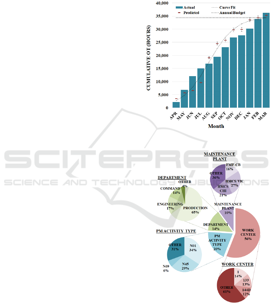
3.4 Model Interpretation
The model output (Holmes, 2020) was used to
generate a budget prediction graph for FY19/20 by
fitting a logistics function for the predicted values
results in Figure 6. Error bars on the predictive
estimates are shown, although they are difficult to
discern due to the fact that they are on the order of
magnitude of the size of the marker at the start of the
FY. After the completion of the fiscal year, the actual
OT data was collected for comparison. As shown, the
final predicted total of OT was within 5% maximum
error of the actual hours reported by the FMF at the
end FY19/20. Due to the smaller number of OT hours
at the beginning of the year and the shape of the
logistics function, the predicted graph indicated that
there should naturally be more difference from the
predicted value early on in the fiscal year. As the
totals increase, the projections become more accurate.
Figure 6: Cumulative OT prediction with logistics function
fit, and actual accrual over FY19/20.
Figure 7: WO attributes as variables of importance for OT,
and top 3 contributors of OT for each.
The WO attributes that are important for
predicting OT accrual are summarized in Figure 7,
which also identifies the top three contributors for
Applying Automated Machine Learning to Improve Budget Estimates for a Naval Fleet Maintenance Facility
591

each. The contributing attribute percentage in Figure
7 correspond to variable of importance calculations
for Model A, obtained from the GBM used as the best
model in H2O autoML. These OT variables of
importance were also similar to those found by
Maybury (Maybury, 2018) when analysing the
primary attributes behind WO maintenance hours for
the FMFs.
4 FUTURE WORK
Based upon the initial findings, supervised and
automated machine learning algorithms available
from H2O were found to be proficient at handling
large, primarily categorical, datasets to build
predictive models. The importance of precautionary
measures required to use automated machine learning
tools effectively, such as, extensive and careful
cleaning of datasets with clear understanding prior to
algorithm input (Ebadi et al., 2019) was noted.
Similarly, the autoML H2O model was found to be
highly interpretable based upon the fundamental
understanding of algorithms used to conduct the
analysis. The predictions resulting from the model
proved to be sufficiently accurate for the purpose of
this study and establish a baseline process for future
predictive models.
To prepare such a model for FMF operations
personnel to use at the beginning of each FY, the data
from the current predicted year would be moved from
Dataset A
p
to Dataset A. A new Dataset A
p
would be
provided shortly after the new FY begins and the
existing model could be re-trained or a new model
using the established process could be developed.
Having more recent data would also allow for the
years with visibly differentiable trends in reporting to
be removed from the input dataset. In-year accrual
data could also be incorporated if the models were
adapted to train on a monthly basis to provide faster
feedback response to the system.
Along with quantifying OT accrual throughout
the FY, knowledge of the specific work which
impacts OT would aid the predictive power of the
model. Ships’ maintenance schedules are known well
in advance, and better association of OT with the
operational maintenance schedule for FMF OT would
provide stronger linkages of when and how much OT
could accrue.
Performing a similar analysis on the OT accrual at
both FMFs would be beneficial, as it would allow for
comparisons in policies and accrual trends. If this
comparison demonstrated that the two FMFs are
similar in their OT accrual patterns, then a larger,
combined dataset could be used to improve the
predictive model.
Finally, operationalizing these algorithms as a
budgeting tool accessible from within enterprise
resource management systems would allow for
decision makers to have updated and readily available
information on the projected OT at the start of a FY,
with adjustments as new data for the FY is in included
in the analysis.
5 CONCLUSIONS
This paper investigated means to improve estimates
of overtime for a naval FMF using automated
machine learning algorithms. Insights to major
variables of importance for OT were explored. Based
on the analysis discussed herein, the following
conclusions are drawn:
A logistics function fit for cumulative OT per
FY provides an improved estimate for annual
OT accrued.
The use of autoML algorithms can improve OT
estimates for the FMF with a maximum error
of 5% observed for FY19/20.
The use of tree-based algorithms can be
informative as to what WO attributes
contribute the most to OT, with quantification
of relative importance over others.
Use of multiple, related datasets enabled
prediction of multiple variables.
The use of such a model would allow decision
makers to prepare more accurate funding estimates
over time – potentially reserving funds for upcoming
critical maintenance tasks or saving funds through
alternative approaches to task management.
ACKNOWLEDGEMENTS
The authors would like to thank the FMF
Comptrollers for their availability and insight, as well
as Mr. Andrew MacDonald for assistance with
manuscript preparation.
REFERENCES
Allison, P., (2012). When can Multicollinearity Safely Be
Ignored? Retrieved 1 October 2020, from
http://statisticalhorizons.com/multicollinearity
Balaji, A., Allen, A., 2018. Benchmarking Automatic
Machine Learning Frameworks. Retrieved from
ICPRAM 2021 - 10th International Conference on Pattern Recognition Applications and Methods
592

https://arxiv.org/abs/1808.06492
Bartek, M. A., Saxena, R. C., Solomon, S., Fong, C. T.,
Behara, L. D., Venigandla, R., et al., 2018. Improving
Operating Room Efficiency: A Machine Learning
Approach to Predict Case-Time Duration. Journal of
the American College of Surgeons, 227(4), 346-354.
Baykasoğlu, A., Öztaş, A., Özbay, E., 2009. Prediction and
multi-objective optimization of high-strength concrete
parameters via soft computing approaches. Expert
Systems with Applications, 36(3, Part 2), 6145-6155.
Desai, R. J., Wang, S. V., Vaduganathan, M., Evers, T.,
Schneeweiss, S., 2020. Comparison of Machine
Learning Methods With Traditional Models for Use of
Administrative Claims With Electronic Medical
Records to Predict Heart Failure Outcomes.
JAMA Network Open. Retrieved from
https://jamanetwork.com/journals/jamanetworkopen/ar
ticle-abstract/2758475
Ebadi, A., Paul, P., Gauthier, Y., Tremblay, S., 2019. How
can automated machine learning help business data
science teams? Paper presented at the 18th IEEE
International Conference on Machine Learning and
Application. Retrieved from https://ieeexplore.ieee.org/
document/8999171
Ellis, N., Davy, R., Troccoli, A., 2015. Predicting wind
power variability events using different statistical
methods driven by regional atmospheric model output.
Wind Energy, 18(9), 1611-1628.
Friedman, J. H., 2001. 1999 Reitz Lecture, Greedy Function
Approximation: A Gradient Boosting Machine. The
Annals of Statistics, 29(5), 1189-1232.
Ganapathi, A., Kuno, H., Dayal, U., Wiener, J. L., Fox, A.,
Jordan, M., et al., 2009. Predicting Multiple Metrics for
Queries: Better Decisions Enabled by Machine
Learning. Paper presented at the 25th International
Conference on Data Engineering. Retrieved from
https://ieeexplore.ieee.org/abstract/document/4812438
Gijsbers, P., LeDell, E., Thomas, J., Poirier, S., Bischl, B.,
Vanschoren, J., 2019. An Open Source AutoML
Benchmark. Paper presented at the 6th ICML
Workshop on Automated Machine Learning. Retrieved
from https://arxiv.org/pdf/1907.00909.pdf
Gohel, H. A., Upadhyay, H., Lagos, L., Cooper, K.,
Sanzetenea, A., 2020. Predictive maintenance
architecture development for nuclearinfrastructure
using machine learning. Nuclear Engineering and
Technology, 52, 1436-1142.
Guanoluisa, D. A. Q., 2020. Design and Implementation of
a Micro-World Simulation Platform for Condition-
Based Maintenance using Machine Learning
Algorithms. University of Toronto.
H2O.ai, (2020). H2O.ai. Retrieved 12 October 2020, from
https://www.h2o.ai/
He, X., Zhao, K., Chu, X., 2020. AutoML: A Survey of the
State-of-the-Art. Knowledge-Based Systems (Preprint
Submission). Retrieved from https://arxiv.org/abs/
1908.00709
Holmes, M., 2020. Predicting Overtime Hours for Fleet
Maintenance Facility Cape Breton (No. DRDC-
RDDC-2020-R071): Defence R&D Canada - Centre for
Operational Research and Analysis.
Kassambara, A., (2018). Logistic Regression Assumptions
and Diagnostics in R. Statistical tools for high-
throughput data analysis Retrieved 1 October 2020,
from http://www.sthda.com/english/articles/36-
classification-methods-essentials/148-logistic
Maybury, D., 2018. Predictive Analytics for the Royal
Canadian Navy Fleet Maintenance Facilities: An
application of data science to maintenance task
completion times (No. DRDC-RDDC-2018-R150):
Defence R&D Canada - Centre for Operational
Research and Analysis.
Naik, J., Dash, P. K., Dhar, S., 2019. A multi-objective
wind speed and wind power prediction interval
forecasting using variational modes decomposition
based Multi-kernel robust ridge regression. Renewable
Energy, 136, 701-731.
Ozturk, S., Fthenakis, V., 2020. Predicting Frequency,
Time-To-Repair and Costs of Wind Turbine Failures.
Energies, 13(5), 1149.
Therneau, T., Atkinson, B., Ripley, B., 2017. Rpart:
Recursive Partitioning and Regression Trees (Version
R package Version 4.1-11).
Truong, A., Walters, A., Goodsitt, J., Hines, K., Bruss, C.
B., Farivar, R., 2019. Towards Automated Machine
Learning: Evaluation and Comparison of AutoML
Approaches and Tools. Retrieved from
https://arxiv.org/pdf/1908.05557.pdf
Applying Automated Machine Learning to Improve Budget Estimates for a Naval Fleet Maintenance Facility
593
