Temporal Transfer Learning for Ozone Prediction based on

CNN-LSTM Model

Tuo Deng

, Astrid Manders

, Arjo Segers

, Yanqin Bai

and Hai Xiang Lin

Delft Institute of Applied Mathematics, Delft University of technology, Mekelweg 4, 2628 CD Delft, The Netherlands

TNO, Climate Air and Sustainability, Utrecht, 3584 CB, The Netherlands

Department of Mathematics, Shanghai University, Shanghai 200444, China

Keywords:

Short-term Ozone Prediction, Transfer Learning.

Abstract:

Tropospheric ozone is a secondary pollutant which can affect human health and plant growth. In this paper,

we investigated transferred convolutional neural network long short-term memory (TL-CNN-LSTM) model to

predict ozone concentration. Hourly CNN-LSTM model is used to extract features and predict ozone for next

hour, which is superior to commonly used models in previous studies. In the daily ozone prediction model,

prediction over a large time-scale requires more data, however, only limited data are available, which causes

the CNN-LSTM model to fail to accurately predict. Network-based transfer learning methods based on hourly

models can obtain information from smaller temporal resolution. It can reduce prediction errors and shorten

run time for model training. However, for extreme cases where the amount of data is severely insufﬁcient,

transfer learning based on smaller time scale cannot improve model prediction accuracy.

1 INTRODUCTION

Tropospheric ozone is formed by the chemical reac-

tion of precursors rather than directly emitted, so it

is classiﬁed as a secondary pollutant (McKee, 1993).

Studies have shown that tropospheric ozone will seri-

ously affect human health (Council et al., 1992) and

plant growth (Iglesias et al., 2006). Therefore, it is

very important to make short-term forecasts for ozone

concentration in the troposphere.

However, it is very difﬁcult to accurately predict

ozone even in the short term. The formation of ozone

is determined by complex chemical reactions. Mean-

while, ozone concentration is easily affected by ozone

precursor emissions (Placet et al., 2000). Common

ozone precursors include nitrogen oxides (NOx) and

volatile organic compounds (VOCs), etc. Various in-

dustrial activities, vehicular trafﬁc, and agricultural

activities generate a large amount of ozone precur-

sors, which can make large changes in ozone concen-

tration in a short time. At the same time, the ozone

concentration is also affected by many meteorologi-

cal factors, such as temperature, wind direction, wind

speed, humidity, solar radiation, etc (Council et al.,

1992). The day-to-day variability in meteorology and

precursor emissions makes it difﬁcult to predict ozone

concentrations.

Currently, there are two main approaches to pre-

dict ozone concentration. The ﬁrst approach is based

on Chemical Transport Models (CTM). For instance,

Lotos-Euros chemical transport model was used to

simulate ozone concentration over Europe (Curier

et al., 2012). The agreement (temporal correlation co-

efﬁcient) between in-situ and modeled ozone concen-

tration is good. However, it is difﬁcult for the model

to capture the ozone peak during the experiment and

it turns to underestimates the daily ozone maximum.

Besides, CTMs also have limitations. It implies that

some other important errors such as the errors in at-

mospheric chemistry mechanism can not be ignored

(Tang et al., 2011). In addition, the resolution is lim-

ited so it cannot resolve all local factors.

At the same time, CTMs often need to simulate

complex physical and chemical processes, which con-

sume a lot of time in calculations. Therefore, some re-

searchers use another approach to predict ozone. The

second approach is to ignore the complex chemical

process in the formation of ozone and directly predict

ozone through data-based machine learning methods.

For instance, regression tree (Zhan et al., 2018) and

Multilayer Perceptron (MLP) (Feng et al., 2019) are

studied for short-term ozone forecast.

Long short-term memory (LSTM) is a widely

used machine learning model (Hochreiter and

Deng, T., Manders, A., Segers, A., Bai, Y. and Lin, H.

Temporal Transfer Learning for Ozone Prediction based on CNN-LSTM Model.

DOI: 10.5220/0010301710051012

In Proceedings of the 13th International Conference on Agents and Artiﬁcial Intelligence (ICAART 2021) - Volume 2, pages 1005-1012

ISBN: 978-989-758-484-8

1005

Schmidhuber, 1997) which can be used in time series

problems. It can capture long-term dependencies in

time-series forecast problems, such as ozone predic-

tion (Eslami et al., 2019). At the same time, Convo-

lutional Neural Network (CNN) is also used by some

researchers in air pollution prediction due to its excel-

lent performance in feature extraction (Sayeed et al.,

2020). It can extract important features in the input

data and improve the performance of model. Many

research also combine CNN with LSTM to extract

temporal and spatial features. CNN-LSTM has been

used in many ﬁelds, such as natural language process-

ing (Wang et al., 2016), medical ﬁeld (Oh et al., 2018)

and industrial area (Zhao et al., 2017).

However, data-based machine learning models re-

quire large amounts of data to train the model. For

large temporal resolution air pollution data sets, it is

often difﬁcult to obtain sufﬁcient data. Transfer learn-

ing (TL) can be a good way to solve this problem. TL

is a research problem in machine learning that focuses

on storing knowledge gained while solving one prob-

lem and applying it to a different but related problem

(Tan et al., 2018). There are few studies in air pol-

lution using transfer learning. Ma (Ma et al., 2019)

used transfer learning to predict particulate matter on

different time scales in China. Compared with par-

ticulate matter, ozone has a more obvious periodicity,

which also provides a basis for our experiments.

This paper aims to use CNN-LSTM to predict

ozone concentration and use Transfer Learning to ﬁt

the new model for larger temporal resolution. We ﬁrst

use CNN-LSTM to ﬁt hourly ozone prediction model.

Compared to other commonly used models in previ-

ous studies, the CNN-LSTM model has smaller pre-

diction errors and it can predict the trend of ozone

well. For daily ozone prediction model, we do not

have sufﬁcient data from daily data set to get accu-

rate result from CNN-LSTM model. With the hourly

model as a basic model, we use transfer learning to

get new daily ozone prediction model, i.e., TL-CNN-

LSTM model. Compared with the LSTM and CNN-

LSTM model, our TL-CNN-LSTM has signiﬁcantly

improved the prediction in terms of root mean square

error, Pearson correlation coefﬁcient and run time for

model training. It implies that transfer learning can

obtain knowledge from a smaller temporal resolution

model and improve model prediction accuracy.

2 DATA AND ANALYSIS

In this section, we describe the processing and anal-

ysis of data. We use interpolation to ﬁx the miss-

ing data and merge the two data sets on different

time scales. Then we conduct correlation analysis for

ozone concentration. For the particularity of time se-

ries, we also need to reconstruct the input data.

2.1 Data Description

The air pollution data that we used is provided by

German environmental agency (UBA). Speciﬁcally,

we use the air pollution data of Eisenh

uttenstadt sta-

tion ’DEBB032’ from 2014 to 2018, which contains

43824 hourly observations. This site was selected in

the experiment because the site has less missing data,

which can reduce the error caused by interpolation.

Each set corresponds to hourly measurements, includ-

ing CO, NO

, NO, NO

, O

, PM

2.5

and SO

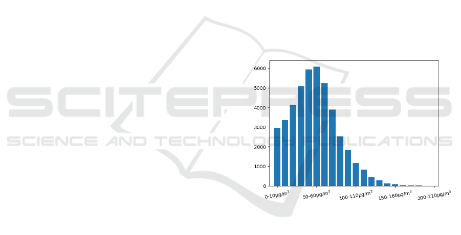
The description of station DEBB032 is in Table 1. To

understand the distribution of ozone, we plot a bar

chart with ozone concentration. We use intervals of

10 µg/m

and show the distribution of ozone in Figure

1. We can see that ozone is concentrated in the range

of 40 to 80 µg/m

. There are only a few cases where

the ozone concentration is higher than 100 µg/m

Figure 1: Distribution of ozone concentration.

In order to simulate the impact of meteorology on

ozone concentration, we also selected the correspond-

ing meteorological data in the E-OBS data set as a

supplement (https://www.ecad.eu/). E-OBS data set

is an ensemble dataset based on gridded observa-

tion of national meteorological institutes and avail-

able on a 0.1 and 0.25 degree regular grid. It covers

the area: 25N-71.5N x 25W-45E. In the experiment,

ﬁve meteorological features were selected, including

the elements daily mean temperature TG, daily min-

imum temperature TN, daily maximum temperature

TX, daily precipitation sum RR and daily averaged

sea level pressure PP. In 0.25°*0.25° data set, we se-

lect the meteorological data of the grid point closest to

the station (52.125°N,12.625°E) at the corresponding

time.

ICAART 2021 - 13th International Conference on Agents and Artiﬁcial Intelligence

1006

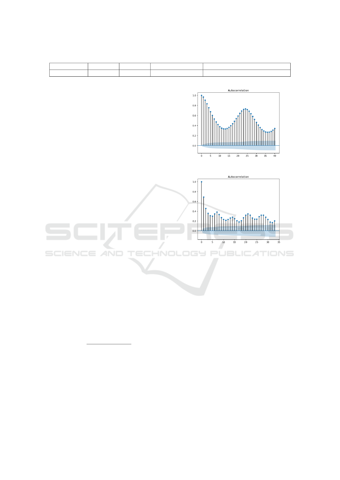
Table 1: Station Description.

No. of station Lat Lon Airbase station type Airbase station ozone classiﬁcation

DEBB032 52.146264 14.638166 industrial suburban

2.2 Data Interpolation and Merging

Due to instrument malfunction and other reasons,

there are missing values in the air pollution data set.

The missing rate of each features is less than 0.5%.

In the experiment, since there is little missing data at

the station, we choose the temporal nearest neighbor

interpolation method to ﬁx the missing value. The

interpolation is implemented through python package

’scipy’.

We then need to unify two different data set be-

cause they have different time scales. Our experiment

requires ozone prediction models for next hour and

next day, so we obtain two different temporal resolu-

tion data set, namely hourly and daily data sets. We

can unify them through the following steps.

Step1: For the daily meteorological data in E-

OBS, we repeat the daily data 24 times and map it

to the hourly air pollution data for that day.

Step2: For hourly ozone concentration data, we

calculate Mean values of the daily maximum 8-h av-

erage (MDA8), which is a commonly used ozone con-

centration evaluation indicator and has a clear thresh-

old.

Step3: For other hourly air pollution data except

ozone, we calculate the daily 24-hour average and

map it to the daily meteorological data.

Through the above three steps, two data sets on

different time scales are obtained. Comparing the size

of the two data sets, the hourly data set has 43824 sets

of data, while the daily data set has only 1826 sets of

data.

2.3 Data Analysis

We use the autocorrelation function to measure the

correlation among ozone on different time scales.

Cov(X(t), X(t + k))

X(t)

X(t+k)

(1)

where X (t) and X(t + k) represent the ozone of one

time series with k time steps difference.

Figures 2 shows the autocorrelation of ozone con-

centration on different time scales. It can be seen that

hourly ozone and daily ozone concentrations are both

periodic. The autocorrelation of hourly ozone con-

centration reaches a peak every 24 time steps, which

matches the daily periodicity. Similarly, we can also

ﬁnd that the daily ozone concentration has a weekly

(a) Hourly ozone

(b) Daily ozone

Figure 2: Autocorrelation coefﬁcient of ozone.

cycle. Although the periods are different, the hourly

ozone and daily ozone concentrations are both peri-

odic and have the same trend. It provides us with a

basis for transfer learning on different time scales.

2.4 Data Transformation in Time Series

In a time series forecast problem, the data is trans-

formed into the following structure.







·· · x

t+d

·· · x

t+1

t+d+1

·· · x

t+2

t+d+2

n+1

·· · x

t+n−1

t+n+d−1







(2)

where {x

, x

, · ·· } is time series data in our exper-

iments, t is the time-step we use in the input and d

is the time-step ahead we want to predict. Each row

is a sample to be trained in the forecast model, and n

rows in the matrix represent a total of n sets of data.

Temporal Transfer Learning for Ozone Prediction based on CNN-LSTM Model

1007

The ﬁrst t columns are used as input features, and the

last column is the output features that need to be pre-

dicted. In the experiment, the number of input time

steps t is determined by actual problems, while the

time step d that needs to be predicted is determined

by requirements.

3 METHODS AND EVALUATION

In this section, we introduce the basic principles of

the CNN-LSTM and Transfer Learning. At the end

of this section, we deﬁne the evaluation criteria of the

model.

3.1 CNN-LSTM

Convolutional neural network (CNN) is a feedforward

network, which is widely used in the ﬁelds of natural

language processing and image processing. The spe-

cial structures of CNN are convolutional layers and

pooling layers. With these layers, main features of

input data are extracted and the parameters required

for model ﬁtting will be greatly reduced. It can solve

the under-ﬁtting problem when the amount of data is

insufﬁcient.

Long short-term memory (LSTM) is a special

RNN model. Compared with RNN, LSTM can solve

the problem of gradient vanish during long-term se-

quence training. A common architecture of LSTM is

composed of a cell and three gates: an input gate, an

output gate and a forget gate. The gates determine

whether the information is discarded or retained.

The basic structure of the CNN-LSTM model in-

cludes CNN layers, pooling layers, LSTM layers and

a ﬁnal fully connected layer. First, the features of in-

put time series are extracted through the CNN layers,

and then the pooling layer is used to retain the main

features while reducing the parameters. The LSTM

layers are trained to ﬁnd the dependence between dif-

ferent time steps in the time series. Finally the output

is predicted through the fully connected layer.

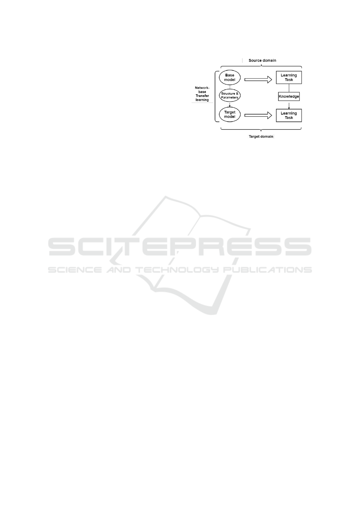
3.2 Transfer Learning

Transfer learning (TL) is a research problem in ma-

chine learning which aims to get knowledge from a

different but related problem. It can solve the prob-

lem of insufﬁcient data in some ﬁelds. The structure

of transfer learning can be seen in Figure 3.

Given a learning task based on target domain, we

can get knowledge from similar task based on source

domain (Tan et al., 2018). Transfer learning can im-

prove the performance of model in target domain, es-

Figure 3: Transfer Learning.

pecially when the amount of data is insufﬁcient. It

is widely used in image recognition and natural lan-

guage processing problems. At present, there are few

studies on transfer learning related to air pollution

prediction.

In our experiments, network based deep transfer

learning is used (Tan et al., 2018). It can reuse the

partial network of basic model that has been trained

in the source domain, such as structures and param-

eters. These information can be transferred into the

model in target domain. In network-based deep trans-

fer learning models, front-layers can be treat as fea-

ture extractor and the remaining layers are the predic-

tor of target task.

In our experiment, hourly ozone prediction model

is used as basic model trained in source domain and

daily ozone prediction model is in target domain.

Knowledge from small time scale is transferred to a

larger time scale. In our CNN-LSTM model, the front

CNN layers and part of LSTM layers are retained

as feature extractors and additional LSTM layers are

added to train the new model.

3.3 Evaluation Criterion

We use root mean squared error (RMSE) and Pear-

son correlation coefﬁcient to evaluate both the hourly

and daily models. For daily ozone prediction model,

we also compare the training time of different model,

which is also an advantage of transfer learning.

For Mean values of the daily maximum 8-h av-

erage (MDA8), there is an evaluation threshold from

World Health Organization (WHO), which is 100

µg/m

. Ozone exceedances can be quantiﬁed through

this threshold. There is no formal threshold for low

ozone concentration, but previous studies have also

found that low ozone concentrations are also harm-

ful to health. Here we select 60 µg/m

as another

threshold. In order to verify whether the model can

accurately predict ozone to the range it belongs to, we

used the above two thresholds to divide the ozone into

ICAART 2021 - 13th International Conference on Agents and Artiﬁcial Intelligence

1008

three categories. Confusion matrix is used to show

the result. The approximate ratio of the three cate-

gories from low to high is 4:5:1. It means that sam-

ples over 100 µg/m

only account for 10% of the total

data, which brings difﬁculties to accurate predictions.

4 EXPERIMENT AND ANALYSIS

In this section, we will introduce in detail the exper-

iments. First, we use CNN-LSTM to predict ozone

concentration for next hour and compare the result

with other commonly used ozone forecast machine

learning models. After that, we use the daily data

set to predict MDA8 for next day. In this case, the

amount of data in this data set is insufﬁcient, which

makes it difﬁcult for the CNN-LSTM model to accu-

rately predict the ozone concentration. Therefore, we

investigate using the hourly model as a basic model

for transfer learning to improve the forecast result.

4.1 One-hour Ozone Prediction

CNN-LSTM is used to train the model for one-hour

ozone forecast. For evaluation, we compare the result

of CNN-LSTM to other commonly used ozone pre-

diction machine learning models in previous studies.

Only hourly data set is used to train the model.

There are still some hyper parameters about neu-

ral networks that need to be determined before model

ﬁtting. As described in Section 2.3, the hourly ozone

concentration is periodic. The ozone concentration

every 24 hours shows a strong autocorrelation. There-

fore, we select the data of past 24 hours as input and

the ozone concentration for the next hour as output.

For each set of inputs, we use all 13 elements as fea-

tures, including 8 air pollution elements and 5 mete-

orological elements. The number of layers and neu-

rons in forecast model is determined through cross-

validation. We set the number of layers of CNN and

LSTM to 1 to 5 and neurons in each layer to 40,

60, 80 and 100, respectively. Through 5-fold cross-

validation, 2 CNN layers with 100 neurons per layer

and 4 LSTM layers with 60 neurons per layer are

ﬁnally selected. Dropout layers are used between

LSTM layers to prevent overﬁtting. One max-pooling

layer is added to the model after CNN layers. At the

same time, we add a fully connected layer contain-

ing a neuron before the output layer. Meanwhile, relu

function is selected as activation function and adam

is selected as optimizer.

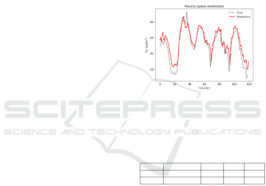
In the hourly data set, we select the ﬁrst 20,000

sets of data as the training set, and the remaining data

as the test set to evaluate the model. We can see the

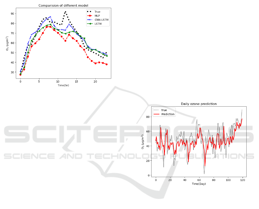
prediction results of the CNN-LSTM model in Figure

4. In Figure 4, we only show the result of last 120

hours in test set. The dotted line is the observation

of ozone concentration, and the red line is the predic-

tion result of CNN-LSTM. From the ﬁgure, we can

see that the red line and the dotted line basically coin-

cide, which means that the CNN-LSTM model can ﬁt

the overall trend of ozone concentration well. At the

same time, the CNN-LSTM model can also simulate

the daily periodic changes of ozone.

Figure 4: CNN-LSTM for 1-h ozone forecast.

We mainly compared CNN-LSTM with three differ-

ent models which are commonly used in previous

studies, namely, Random Forest (Feng et al., 2019),

MLP (Sayeed et al., 2020) and LSTM (Eslami et al.,

2019). The RMSE and Pearson correlation coefﬁcient

of each model are shown in Table 2.

Table 2: Performance of different model for ozone forecast.

Model CNN-LSTM LSTM MLP RF

RMSE 9.05 11.91 13.81 13.25

Corr 0.96 0.95 0.95 0.90

It can be seen from Table 2 that all four models can

simulate the trend of ozone well. Among them, the

prediction result of the random forest method (500

regression trees) has the lowest correlation coefﬁ-

cient with the observation, only 0.90. Comparing the

RMSE of four models, we can ﬁnd that CNN-LSTM

can get the smallest RMSE, only 9.05. It can get more

accurate prediction results than the other three mod-

els.

Besides, we also compared with other ensemble

methods, such as gradient boosting (500 regression

trees). Their performance is similar to the random for-

est, so we did not list them in Table 2. We also com-

pared our model with the python package ’Prophet’,

which is commonly used in time series prediction

Temporal Transfer Learning for Ozone Prediction based on CNN-LSTM Model

1009

problem (Taylor and Letham, 2018). However, since

the input for ’Prophet’ only contains ozone data, the

model can only simulate the general trend of ozone

and cannot accurately predict the ozone concentra-

tion. Its RMSE is above 20, much larger than our

model.

Figure 5: Prediction of different models.

In order to compare the three models with similar re-

sults, namely MLP, LSTM and CNN-LSTM, we show

the ozone peak part of the day in Figure 5. Although

all three models tend to underestimate the daily max-

imum value of ozone concentration, the CNN-LSTM

model still performs the best among them. In com-

parison, CNN-LSTM has obvious advantages in the

prediction of daily ozone peaks.

4.2 Transfer Learning based Daily

Ozone Prediction

It is shown in the previous section that CNN-LSTM

is effective for 1-hour ozone prediction. In the fol-

lowing, we use daily data set to ﬁt new models for

daily ozone prediction. However, a larger time scale

will result in greater changes in ozone at adjacent time

steps. Meanwhile, less data are available for training.

From section 2.2, we can know that the hourly data

set has more than 40,000 sets of data, while the daily

data set has only 1826 sets of data. In this section,

we use houly CNN-LSTM ozone prediction model

as a basic model to train the daily ozone prediction

model through transfer learning, namely TL-CNN-

LSTM ozone prediction model.

For the daily ozone concentration data set, al-

though MDA8 do not have the same cycle as the

hourly ozone concentration, the overall trend are sim-

ilar. At the same time, the CNN-LSTM model can

effectively extract the features in the time series. It

makes it possible for us to retain features extracted

from front-layers of hourly model and use transfer

learning to improve the performance of daily model.

We select the ﬁrst 1200 sets of data in the daily data

set as the training set, and the remaining data as the

test set. In order to show the effect of transfer learn-

ing, we keep the parameters the same as the hourly

model in the experiment.

In the training process of TL-CNN-LSTM model,

one new parameter is the number of frozen layers ex-

tracted from the basic model. It determines how many

layers of the base model needs to be retained. Starting

from the ﬁrst CNN layer, the parameters in the hourly

CNN-LSTM model are retained layer by layer. At the

same time, up to 4 LSTM layers are added to the new

model after frozen layers. Table 3 shows that when 2

CNN layers and 2 LSTM layers are retained, the pre-

diction result obtained by transfer learning model is

the best. They have the least RMSE and the largest

correlation coefﬁcient. It suggests that too many or

too few retained features can both make the target

model perform worse in transfer learning. The result

of TL-CNN-LSTM model is shown in Figure 6.

Figure 6: TL-CNN-LSTM for 1-day ozone forecast.

We also compare TL-CNN-LSTM with LSTM and

CNN-LSTM, which perform well in the previous

hourly forecast models. From Table 4, we can

ﬁnd the negative impact of insufﬁcient data on the

above model. All three models have big RMSE in

the daily model, while TL-CNN-LSTM performs the

best. Compared with CNN-LSTM, the RMSE in the

prediction results of TL-CNN-LSTM is reduced by

21%, and the correlation coefﬁcient is increased by

13%. At the same time, the training time of daily

model is also greatly reduced through transfer learn-

ing. The run time to train TL-CNN-LSTM is only

about half of CNN-LSTM. It implies that the features

in the hourly CNN-LSTM model can be extracted and

transferred by transfer learning, which can improve

the predictive performance of the target model with

larger time scale.

ICAART 2021 - 13th International Conference on Agents and Artiﬁcial Intelligence

1010

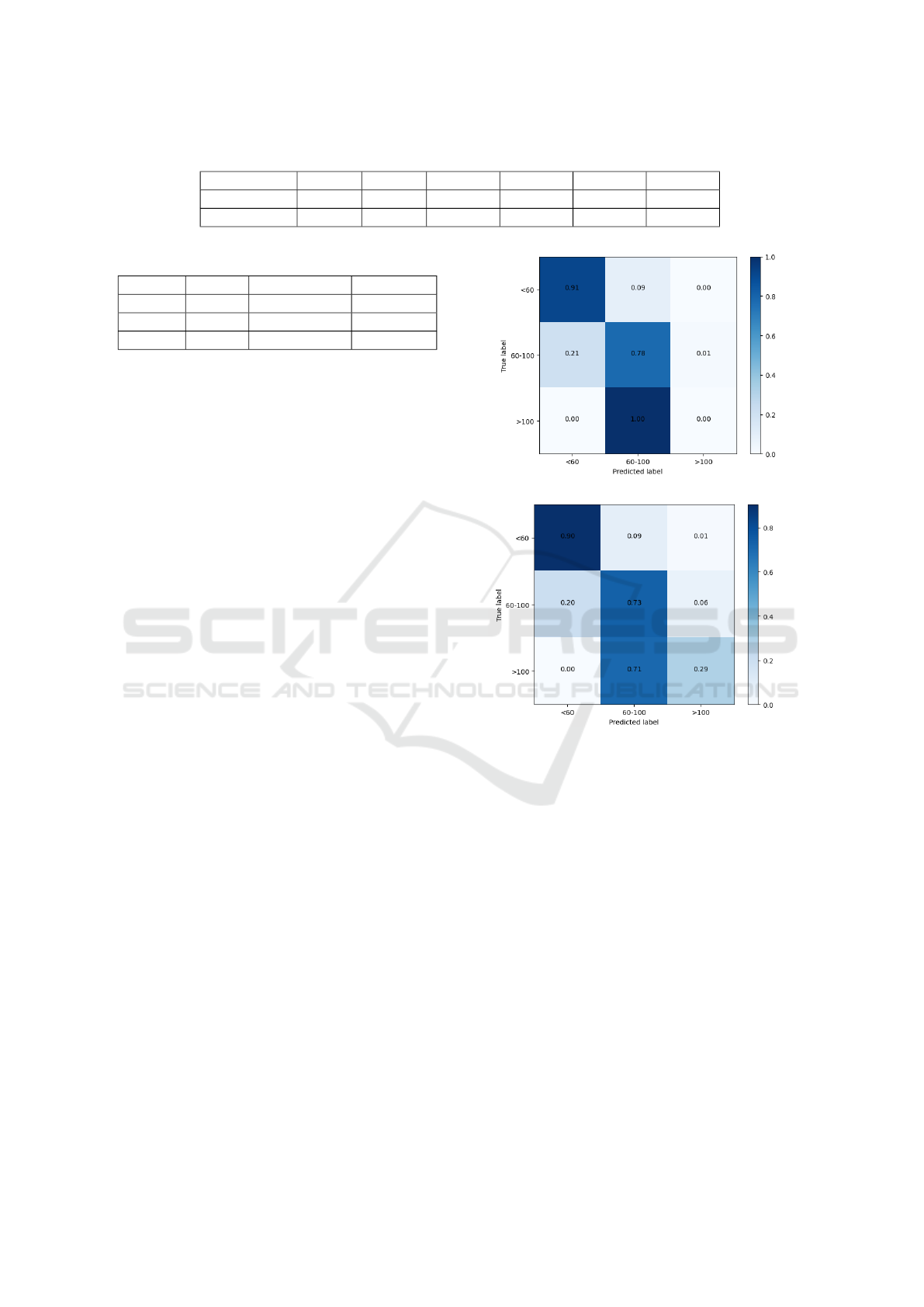
Table 3: Result of TL-CNN-LSTM with different frozen layers.

Frozen layer CNN-1 CNN-2 LSTM-1 LSTM-2 LSTM-3 LSTM-4

RMSE 20.54 18.40 15.55 14.92 15.08 16.82

Corr 0.71 0.72 0.80 0.81 0.80 0.74

Table 4: Comparison of different model.

Model LSTM CNN-LSTM TL-Model

RMSE 19.14 18.83 14.92

Corr 0.70 0.71 0.81

Time(s) 306 168 75

However, the model still has shortcomings in the daily

peak forecasting due to the serious lack of data in this

part. As described in Section 3.3, we divide MDA8 in

the test set into three classes. We evaluate the model’s

prediction accuracy for the range of ozone concentra-

tion through confusion matrices, which can be seen in

Figure 7.

In general, events of high ozone concentration are

particularly important which require our attention, be-

cause these have direct impact on human health. It

can be seen from Figure 7 that for low and medium

ozone concentrations, the CNN-LSTM model can al-

ready predict its range accurately. Whereas, the CNN-

LSTM model do not predict ozone concentrations

higher than 100µg/m

at all, while TL-CNN-LSTM

can accurately predict 29% of this part of the data.

As mentioned in section 3.3, only around 10% of

ozone data is higher than 100µg/m

, which means

only around 2000 samples in the hourly data set and

100 samples in the daily data set in this class. Nei-

ther the transfer learning method nor the CNN-LSTM

model can effectively extract relevant features.

For transfer learning, it is difﬁcult to improve the

prediction accuracy of extreme events, that is, ozone

exceedances in our experiments. For this problem,

one possible solution is to simulate more high daily

ozone concentration data through methods such as re-

sampling, which has been proven to be effective in

visibility prediction (Deng et al., 2019). However,

ozone data simulation will be more difﬁcult because

the ozone concentration is periodic.

5 CONCLUSIONS

We use two data sets with different time scale to

predict ozone concentration with CNN-LSTM model

and network-based transfer learning methods. CNN-

LSTM is used to predict ozone concentration for next

hour with hourly data set. Compared with three com-

monly used models in previous studies, namely, RF,

(a) CNN-LSTM

(b) TL-CNN-LSTM

Figure 7: Confusion Matrix.

MLP and LSTM, CNN-LSTM performs the best in

both overall trend and accuracy. In particular, for the

prediction of peak ozone concentration, CNN-LSTM

performs signiﬁcantly better than other models. It

shows that CNN-LSTM model can be used in hourly

ozone prediction problems and performs well.

We also used daily ozone data set to predict ozone

for next day. CNN-LSTM model is used and the re-

sult is improved through the transfer learning method

based on hourly CNN-LSTM model. In a daily

time scale, the number of samples is greatly dimin-

ished. Insufﬁcient training data leads to the CNN-

LSTM model with a large error in daily ozone pre-

diction problem. The network-based transfer learn-

ing method can obtain the extracted features from the

CNN-LSTM model of a smaller time scale and im-

proves the performance of target model. Compared

to daily CNN-LSTM model, TL-CNN-LSTM model

Temporal Transfer Learning for Ozone Prediction based on CNN-LSTM Model

1011

can reduce the RMSE by 21% and training time by

55%.

In current practice, we still need to use the tra-

ditional chemical transport model to predict ozone,

because it is more accurate in case of high ozone

concentrations. Compared to the chemical transport

model, our TL-CNN-LSTM model is more ﬂexible

and can be applied to various local problems, such as

ozone concentration prediction at a single site. At the

same time, the machine learning method greatly saves

the time and resource consumption of model training.

However, in the case of ozone exceedances, the severe

lack of relevant samples makes even transfer learn-

ing model can not predict accurately. Network-based

transfer learning only enables the target model to ob-

tain main features from similar models, and a certain

amount of data corresponding to cases of interest is

still needed to train the new model with different pa-

rameters. To solve this problem, we can add more

input samples by re-sampling or other methods. In fu-

ture research, we will investigate adding other ozone-

related elements to the input data, such as predicted

future temperature, to increase the accuracy of model

predictions. At the same time, our current experiment

is only based on the data from one site. We will use

data from more sites to train and optimize the model

through spatial transfer learning.

ACKNOWLEDGEMENTS

We thank the German environmental agency for the

air pollution data which is used in the case study for

training the neural network models.

REFERENCES

Council, N. R. et al. (1992). Rethinking the ozone prob-

lem in urban and regional air pollution. National

Academies Press.

Curier, R., Timmermans, R., Calabretta-Jongen, S., Eskes,

H., Segers, A., Swart, D., and Schaap, M. (2012).

Improving ozone forecasts over europe by synergis-

tic use of the lotos-euros chemical transport model

and in-situ measurements. Atmospheric environment,

60:217–226.

Deng, T., Cheng, A., Han, W., and Lin, H.-X. (2019). Vis-

ibility forecast for airport operations by lstm neural

network. In ICAART (2), pages 466–473.

Eslami, E., Choi, Y., Lops, Y., and Sayeed, A. (2019). A

real-time hourly ozone prediction system using deep

convolutional neural network. Neural Computing and

Applications, pages 1–15.

Feng, R., Zheng, H.-j., Zhang, A.-r., Huang, C., Gao,

H., and Ma, Y.-c. (2019). Unveiling tropospheric

ozone by the traditional atmospheric model and ma-

chine learning, and their comparison: A case study in

hangzhou, china. Environmental pollution, 252:366–

378.

Hochreiter, S. and Schmidhuber, J. (1997). Long short-term

memory. Neural computation, 9(8):1735–1780.

Iglesias, D. J., Calatayud,

A., Barreno, E., Primo-Millo,

E., and Talon, M. (2006). Responses of citrus plants

to ozone: leaf biochemistry, antioxidant mechanisms

and lipid peroxidation. Plant Physiology and Bio-

chemistry, 44(2-3):125–131.

Ma, J., Cheng, J. C., Lin, C., Tan, Y., and Zhang, J. (2019).

Improving air quality prediction accuracy at larger

temporal resolutions using deep learning and trans-

fer learning techniques. Atmospheric Environment,

214:116885.

McKee, D. (1993). Tropospheric ozone: human health and

agricultural impacts. CRC Press.

Oh, S. L., Ng, E. Y., San Tan, R., and Acharya, U. R.

(2018). Automated diagnosis of arrhythmia using

combination of cnn and lstm techniques with vari-

able length heart beats. Computers in biology and

medicine, 102:278–287.

Placet, M., Mann, C., Gilbert, R., and Niefer, M.

(2000). Emissions of ozone precursors from stationary

sources:: a critical review. Atmospheric Environment,

34(12-14):2183–2204.

Sayeed, A., Choi, Y., Eslami, E., Lops, Y., Roy, A., and

Jung, J. (2020). Using a deep convolutional neural net-

work to predict 2017 ozone concentrations, 24 hours

in advance. Neural Networks, 121:396–408.

Tan, C., Sun, F., Kong, T., Zhang, W., Yang, C., and Liu,

C. (2018). A survey on deep transfer learning. In

International conference on artiﬁcial neural networks,

pages 270–279. Springer.

Tang, X., Zhu, J., Wang, Z., and Gbaguidi, A. (2011). Im-

provement of ozone forecast over beijing based on en-

semble kalman ﬁlter with simultaneous adjustment of

initial conditions and emissions. Atmospheric Chem-

istry and Physics, 11(24):12901.

Taylor, S. J. and Letham, B. (2018). Forecasting at scale.

The American Statistician, 72(1):37–45.

Wang, J., Yu, L.-C., Lai, K. R., and Zhang, X. (2016).

Dimensional sentiment analysis using a regional cnn-

lstm model. In Proceedings of the 54th Annual Meet-

ing of the Association for Computational Linguistics

(Volume 2: Short Papers), pages 225–230.

Zhan, Y., Luo, Y., Deng, X., Grieneisen, M. L., Zhang, M.,

and Di, B. (2018). Spatiotemporal prediction of daily

ambient ozone levels across china using random for-

est for human exposure assessment. Environmental

Pollution, 233:464–473.

Zhao, R., Yan, R., Wang, J., and Mao, K. (2017). Learn-

ing to monitor machine health with convolutional bi-

directional lstm networks. Sensors, 17(2):273.

ICAART 2021 - 13th International Conference on Agents and Artiﬁcial Intelligence

1012