Locating Datacenter Link Faults with a Directed Graph Convolutional
Neural Network
Michael P. Kenning, Jingjing Deng, Michael Edwards and Xianghua Xie
Swansea University, U.K.
csvision.swan.ac.uk
Keywords:
Graph Deep Learning, Fault Detection, Datacenter Network, Directed Graph, Convolutional Neural Network.
Abstract:
Datacenters alongside many domains are well represented by directed graphs, and there are many datacenter
problems where deeply learned graph models may prove advantageous. Yet few applications of graph-based
convolutional neural networks (GCNNs) to datacenters exist. Few of the GCNNs in the literature are explicitly
designed for directed graphs, partly owed to the relative dearth of GCNNs designed specifically for directed
graphs. We present therefore a convolutional operation for directed graphs, which we apply to learning to
locate the faulty links in datacenters. Moreover, since the detection problem would be phrased as link-wise
classification, we propose constructing a directed linegraph, where the problem is instead phrased as a vertex-
wise classification. We find that our model detects more link faults than the comparison models, as measured
by McNemar’s test, and outperforms the comparison models in respect of the F
1
-score, precision and recall.
1 INTRODUCTION
The convolutional neural network’s (CNN) represen-
tational power is owed to its small kernels, permitting
a small set of parameters to compose low-level fea-
tures over a sequence of layers into higher-order sig-
nals. The kernel’s structure however restrictsCNNs
are restricted to regular structures, such as images and
video, precluding their direct use on a great number of
natural domains exist in non-Euclidean domains.
A great effort therefore has been expended in gen-
eralizing CNNs to irregular domains. One structure
that represents irregular domains well is the graph. As
with a signal over a grid of pixels, a redesigned ker-
nel can be convolved over a graph signal both in the
spectral (Bruna et al., 2014; Defferrard et al., 2016;
Kipf and Welling, 2017; Levie et al., 2019) and spa-
tial domains (Niepert et al., 2016; Gilmer et al., 2017;
Monti et al., 2017; Hamilton et al., 2017). Few meth-
ods however extend the CNN to directed graphs (Ma
et al., 2019; Cui et al., 2020). Fewer methods ex-
ist for learning representations on graph edges, both
with and without linegraphs (Klicpera et al., 2020;
Jørgensen et al., 2018; Chen et al., 2019).
Datacenters readily exhibit graph structure, espe-
cially a directed graph structure. But while there are
many applications of machine learning to datacenter
problems (Wang et al., 2018; Srinivasan et al., 2019;
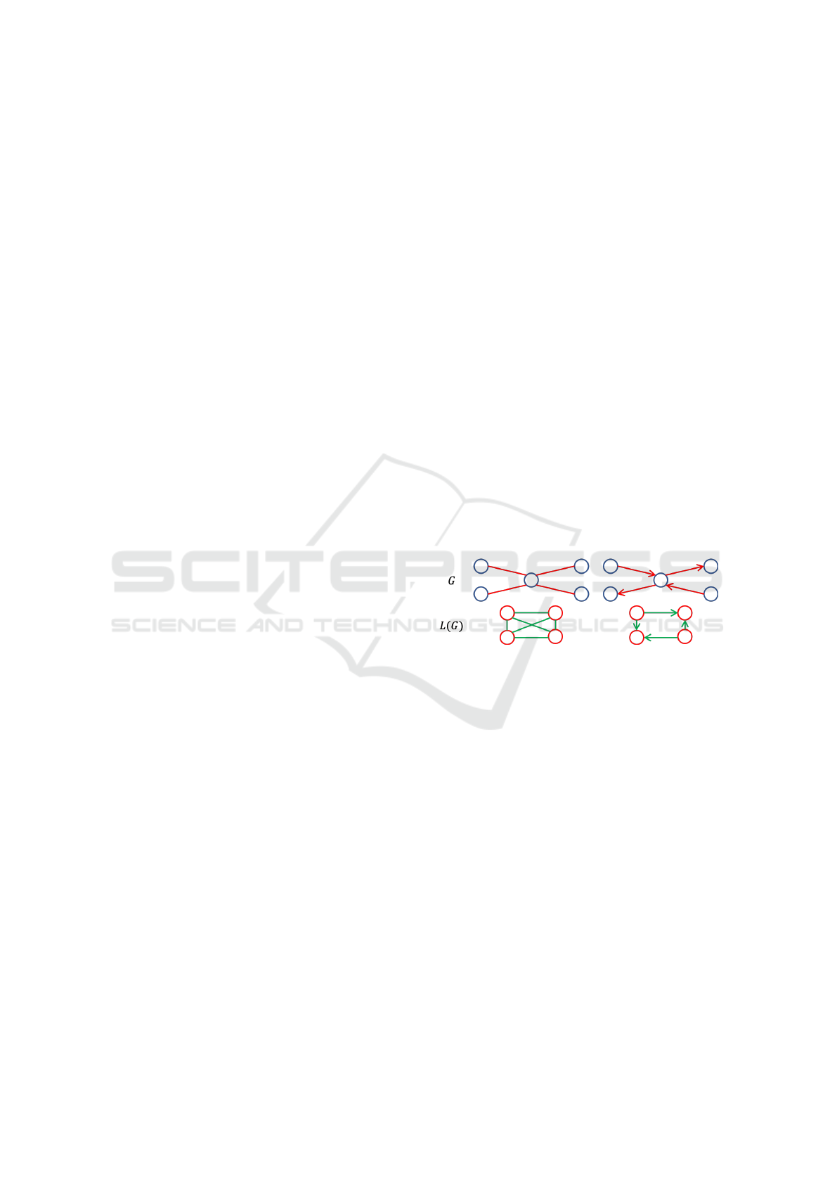
Figure 1: Constructing a linegraph from its underlying
graph. On the left-hand side the two graphs are undirected,
and on the right-hand side the two are directed.
Ji et al., 2018; Xiao et al., 2019), very few use graph-
based convolutional neural networks (GCNNs) (Pro-
togerou et al., 2020; Li et al., 2020). To the best of
our knowledge, none represents the datacenter as a
directed graph
In this paper we describe a GCNN that can be
applied to directed graphs. The model we con-
struct, the directed graph convolutional neural net-
work (DGCNN), is composed of convolutional layers
use edge orientation to aggregate local graph signals.
We train the DGCNN to locate the link faults in a dat-
acenter, represented by a directed linegraph, a way of
representing edge signals with few antecedents Chen
et al. (2019). We use in silico data generated the simu-
lator developed by Arzani et al. (2018), the advantage
of in silico data being that it permits an easy identifi-
cation of the ground-truth.
To summarize, our paper contributes the follow-
ing:
312
Kenning, M., Deng, J., Edwards, M. and Xie, X.
Locating Datacenter Link Faults with a Directed Graph Convolutional Neural Network.
DOI: 10.5220/0010301403120320
In Proceedings of the 10th International Conference on Pattern Recognition Applications and Methods (ICPRAM 2021), pages 312-320
ISBN: 978-989-758-486-2
Copyright
c
2021 by SCITEPRESS – Science and Technology Publications, Lda. All rights reserved

• An approach to learning on the edges of directed
graphs by constructing a directed linegraph from
a directed graph.
• A technique to learn feature representations on di-
rected graphs, by altering the definition of the ag-
gregation step of a spatial graph neural network.
• A new application of graph neural networks to lo-
cating link faults in datacenters.
In Section 2 we outline previous work on graphs
and machine-learning applications to datacenters. In
Section 3 we present our technique for learning on
a directed linegraph. In Section 4 we describe our
dataset, the model’s and comparison models’ imple-
mentation, the experimental conditions, and the met-
rics on which we assess our model against the com-
parison models. The results are discussed in Sec-
tion 5, and we conclude the paper in Section 6.
2 RELATED WORK
2.1 Graph Convolutional Neural
Networks
As acknowledged in early work (Sperduti and Starita,
1997), fully connected neural networks do not ap-
propriately process structured information (Bronstein
et al., 2017). Models that leverage graph structure
gain an analytical power: a graph can encode the re-
lational structure of a signal, and so bestow a model
with helpful inductive biases (Battaglia et al., 2018).
There are two ways of defining convolution on a
graph: spectrally and spatially. GCNNs are hence de-
scribed as either spectral or spatial. We outline several
such techniques of both kinds below.
Spectral Convolution on Graphs. Bruna et al.
(2014) proposed the first graph-based convolutional
neural network that uses the spectral definition of con-
volution. A graph may be represented as a Laplacian
matrix. For undirected graphs, this matrix is symmet-
ric and positive semidefinite, so we are able to ob-
tain a full set of eigenvectors by eigendecomposition.
These eigenvectors can then be used to project graph
signals into the spectral domain, where we can ap-
ply the Hadamard product. This would yield as many
parameters as vertices of the graph, so Bruna et al.
proposed learning spline coefficients that are interpo-
lated to form a filter, in turn yielding smoother fil-
ters that correspond to localized convolutional filters
in the spatial domain (Shuman et al., 2013).
Owing to the O (|V |
2
) computational cost of com-
puting the eigenvectors, where V is the vertex set,
later research focused on efficient approximations of
the spectral filter. Defferrard et al. (2016) proposed
an approximation using Chebyshev polynomials, re-
ducing the computational cost of filtering to O(k|E|),
where k is the order of the Chebyshev polynomial
and E is the edge set. Chebyshev polynomials are
ill-suited to community detection problems, however,
as they cannot produce low-order, localized, narrow-
band filters. Levie et al. (2019) proposed Cayley poly-
nomials instead, the computational cost of which is
O(|V |).
Bruna et al.’s method and the subsequent approx-
imations are however limited to undirected graphs,
owing to the requirement that the graph Laplacian ma-
trix be symmetric. This is not possible with directed
graphs, as the adjacency matrix is not symmetric.
Two methods have been proposed to overcome this
problem. Ma et al. (2019) used the Perron-Frobenius
theorem to extract the Perron vector from the proba-
bility matrix of the directed graph, which can then be
used to construct a symmetric Laplacian matrix. To
learn on directed signed graphs on the other hand, Cui
et al. (2020) constructed a signed Laplacian matrix,
which is used to implement convolution in a similar
manner as in Bruna et al.’s work. Both these tech-
niques require the directed graph to be strongly con-
nected, meaning that there should be a path from ev-
ery vertex to every other vertex in the graph.
The spectral methods we described above have
several disadvantages. Firstly they assume a fixed
graph, as the filtering is defined on the graph Lapla-
cian, which changes as the graph’s structure changes.
Consequently a model based on a Laplacian matrix
cannot be applied to dynamic domains. Secondly, it
is unclear whether spectral techniques work on graph
localization problems where several independent sig-
nals exist. Thirdly, as mentioned above, the former
techniques do not work on directed graphs, while the
latter two only work on strongly connected graphs.
On the contrary, the spatial techniques we discuss be-
low can accommodate these properties.
Spatial Convolution on Graphs. Spatial con-
volution on graphs works locally on each vertex,
like convolution on an image centers on each pixel.
Each technique requires us to define a vertex’s
neighborhood and the function we use to filter the
neighborhood’s signals. The neighborhood is difficult
as there is no immediately meaningful way to describe
a locality in a graph unless defined already by the do-
main The filtering function is yet more difficult. The
placement of pixels in an image is fixed and a neigh-
Locating Datacenter Link Faults with a Directed Graph Convolutional Neural Network
313

borhood has the same structure everything. A
CNN hence binds its kernels’ parameters to positions
in a neighborhood by their offset from the center. A
graph’s vertices however have no natural ordering
(unless bestowed by the domain); the neighborhood
sizes may also vary between each vertex. Simply
binding a graph model’s parameters to a neigh-
borhood’s vertices is hence troublesome, and must
either be managed with additional procedures or
circumvented. Graph models differ primarily in the
way they handle the signals.
Niepert et al. (2016) were among the earliest
to generalize CNNs to graphs. Their technique,
PATCHY-SAN, consists of three stages: selection, ag-
gregation and normalization. In the selection stage, a
labeling procedure ranks a graph’s vertices and selects
the top w vertices, mimicking striding in a CNN. Then
a k-large neighborhood around each vertex is aggre-
gated, subject to a further labeling. Finally each sub-
graph around the vertices is normalized. PATCHY-
SAN can be extended to operate on edge attributes.
Gilmer et al. (2017) proposed the message-
passing neural network. Each vertex’s state is updated
by a so-called message, consisting of a summation
of a message function over the one-hop neighbors’
edge and vertex attributes. The message function, be-
ing a summation, is commutative, but vulnerable to
large variations in a vertex’s degree. The final layer is
a readout function, commutative on the graph’s ver-
tices.
Monti et al. (2017) developed a convolution
layer that maps graph neighborhoods into a pseudo-
coordinate space of a mixture of learned Gaussian dis-
tributions. The posterior probabilities thereby act as
weights to each vertex in the neighborhood, the re-
sults of which are passed through an activation layer.
Learning vertex weightings indirectly via Gaussian
distributions means this technique copes well with
variations in the degree of the vertex.
Hamilton et al. (2017) avoided separately weight-
ing the features of vertices of a neighborhood by ag-
gregating the one-hop neighborhood and applying a
commutative function and an activation layer. With
a mean aggregator it is similar to Kipf and Welling’s
Graph Convolutional Network (GCN), which by con-
trast accepts weighted graphs, too.
A few techniques exist for learning on directed
graphs and on directed linegraphs of graphs. Klicpera
et al. (2020) used directional messages and second-
order features on the graph to regress on molecular
properties. Jørgensen et al. (2018) proposed a tech-
nique to incorporate edge information in the learning
for a regression on molecular properties, while Chen
et al. (2019) proposed a method to learn edge repre-
sentations on a directed linegraph to inform a commu-
nity detection problem on the vertices of the graph.
2.2 Locating Faults in Datacenters
A failure in a datacenter can exist anywhere on the
multitude of machines and links that comprise it. A
network administrator must collate and interrogate
many sources of information to determine the location
of problems (Gill et al., 2011). Manually this is time-
consuming and difficult, and potentially very costly
problem when responses need to be quick to reduce
disruption to clients. Automating the interrogation of
logs with an algorithm is quicker. For example, Zhang
et al. (2005) postulated the loads on individual links
as a linear transformation of unknown traffic elements
that is inverted to discover the anomalies.
There are also monitoring systems available that
help in diagnosing datacenter faults expeditiously.
Pingmesh (Guo et al., 2015) monitors faults on dis-
tributed servers by running an agent on its every
server to measure the latency of the network. 007
(Arzani et al., 2018) by contrast has at every host an
agent that traces the path of detected TCP retransmis-
sion errors, on which several algorithms can be run to
rank the links by likelihood of fault.
Machine-learning algorithms are particularly suit-
able to these problems (Wang et al., 2018). Srinivasan
et al. (2019) for instance located link disconnections
in an Internet-of-Things (IoT) network of up to 100
nodes using one such model, attaining a high detec-
tion rate in silico. Ji et al. (2018) used a CNN to
scan log files to predict future network faults. Xiao
et al. (2019) applied a CNN to detect intrusive behav-
ior among network traffic.
But despite the power that graphs offer in ex-
plicitly representing the structure of datacenters, they
are scarcely used in the literature. Protogerou et al.
(2020) applied a graph network to detect denial-of-
service attacks in an IoT network; whereas Li et al.
(2020) applied a similar network to optimize a data-
center’s traffic-flow. The novelty of our work is that
we use both a GCNN and represent the datacenter as a
directed graph to locate link faults in a datacenter. To
the best of our knowledge, there are no such examples
of work in the literature.
3 METHOD
Problem Description. Failures in a datacenter can
cost network operators and end-users time and money.
There are myriad causes of failures in a datacenter.
ICPRAM 2021 - 10th International Conference on Pattern Recognition Applications and Methods
314

The aim of the engineer is to identify and fix the most
unreliable machines and links in the datacenter. De-
tecting these faults is non-trivial. Network operators
must assess a plethora of machines and many more
links, drawing on multiple indicators from across the
network to track the health of the network. The task of
the operator is to prioritize the most severe incidents
(Gill et al., 2011).
One indication of a fault is packets dropping at
an abnormal rate, which is picked up by host ma-
chines: When packet-drops occur in the middle of
a TCP transmission, the destination machine sends a
TCP retransmission error to the originating machine
to request same packet again. Accordingly Arzani
et al. (2018) developed the 007 system to use a dat-
acenter’s hosts to determine the paths along which a
retransmission error occurred, and assign a score of
blame to each link. The system then uses the hosts’
aggregated blame scores to find the most probable lo-
cations of link faults.
But it is not so simple as finding k links assigned
the greatest blame. Faults displace traffic and cause
collateral faults elsewhere; genuinely faulty links are
lost in a mire of overburdened links. For this reason,
it is more helpful to understand the context of a link’s
blame score than to look at scores in isolation. Hence
understanding the structure of the datacenter is essen-
tial in locating faults.
Our objective is to design a graph-based model
that can predict the faulty links in a datacenter.
Graphs represent datacenters well. By incorporating
the graph structure into a model, we are able to pro-
duce a model that accounts for contextual informa-
tion.
Graph-theoretical Definitions. A graph G =
hV,Ei is defined by the sets of vertices or nodes
V = V (G) and edges E = E(G). If two vertices
x,y ∈ V are adjacent, they are incident to an edge
{x,y} = xy = e ∈ E. Every edge in a graph is therefore
incident to two endvertices. For undirected graphs, E
is a set of unordered pairs, meaning xy = yx ∈ E; but
for directed graphs E is a set of ordered pairs, mean-
ing xy 6= yx. Directed edges (x,y) are therefore inci-
dent to a startvertex x and endvertex y. If xy, yx ∈ E
is xy has an inverse edge yx. A directed graph where
every edge has an inverse is called symmetric. A di-
rected graph where every vertex is reachable from ev-
ery other vertex is strongly connected (see Fig. 1 for
an example of a weakly connected graph).
The order of the graph is |G| = |V | = n, the num-
ber of vertices, while the size of the graph is |E|, the
number of edges. In an undirected graph, a vertex’s
degree d(x) is the number of adjacent vertices to x.
The minimum and maximum degree of a graph G are
denoted respectively δ(G) and ∆(G). In a directed
graph, the degree of a vertex x is the sum of the in-
degrees d
−
(x) = |
{
(y,x)|(y, x) ∈ E
}
| and out-degrees
d
+
(x) = |
{
(x,y)|(x,y) ∈ E
}
|.
The neighborhood of a target vertex Γ(x) consists
of its adjacent vertices and incident edges, the one-
hop neighbors. The concept of a neighborhood can be
expanded beyond the first hop to include those k hops
away, which we denote Γ
k
(x) ⊃ Γ
1
(x) = Γ(x) for k >
1. The neighborhood of a vertex in a directed graph
can be factored into neighbors incident to its in- and
out-edges: Γ(x) = Γ
−
(x) ∪ Γ
+
(x). The neighborhood
can thus be conceived as a subgraph, with the order
and size of it defined equivalently.
A graph can be represented in matrix form in a
number of ways, requiring an indexing of the vertices.
An adjacency matrix A is a binary matrix where each
non-zero entry marks an adjacency between two ver-
tices: ∀i j ∈ V,A
i j
= 1. A degree matrix D is a diag-
onal matrix where the diagonal records the degree of
each vertex, D = diag(A1). A directed graph’s adja-
cency matrix is asymmetric. It has two degree matri-
ces corresponding to the in- and out-degrees, defined
as D
−
= diag(A
>
1) and D
+
= diag(A1) respectively.
An undirected linegraph L(G) is defined on an un-
derlying undirected graph G. It is an ordered pair
hV
L
,E
L
i, where V
L
:= E(G). Consequently there is a
bijective and hence invertible mapping from the edge
set of G to the vertex set of L(G). Two vertices in the
linegraph α, β ∈ L(G) are adjacent if their edges in the
underlying graph G have an endvertex in common. A
directed linegraph (Aigner, 1967) is constructed in a
more constrained manner. Two vertices in a directed
linegraph are adjacent iff for the two edges in the un-
derlying directed graph the endvertex of one edge is
identical to the startvertex of the other. (See Fig. 1 for
a visual illustration of the construction of a directed
and undirected linegraph.) The adjacency and degree
matrices of the undirected and directed linegraphs are
formed similarly to those of their underlying graphs;
we denote them A
L
and D
L
.
A m-dimensional signal on a graph or linegraph
is the codomain of a mapping from its vertices to the
real vector space f : V → R
m
. The signal may also
be a mapping from a graph’s edges f : E → R
m
. The
graph thus describes the structure of the signal. Many
observed signals may share the same structure. Our
dataset consists of a set of observations of a structured
signal on a linegraph. Each observation is therefore a
separate mapping. We often refer to a vertex’s signal
simply as the vertex.
Locating Datacenter Link Faults with a Directed Graph Convolutional Neural Network
315

A Datacenter as a Graph. A datacenter can be eas-
ily represented as a graph if we consider each machine
to be a vertex and draw edges between machines if
they are connected. In our case we use an unweighted
graph. As mentioned above, each connection between
a pair of machines consists of an uplink and down-
link, two opposing flows of traffic, which can be rep-
resented as directed edges in a symmetric directed
graph.
On top of this unweighted graph, we can build
a directed linegraph, where each vertex represents a
link in the datacenter. The linegraph of the data-
center’s graph therefore represents the second-order
structure of the datacenter, the adjacency of the links.
A path of vertices in the graph represents the passage
of a packet through the datacenter. We do not join in-
verse edges in the directed linegraph for two reasons.
On the practical side, the an edge’s inverse belongs to
both the in- and out-neighbors: either count it dou-
bly or exclude it. From the point of view of the do-
main, an edge’s inverse is irrelevant, as a packet that
is routed up or down the datacenter will not traverse
a link it has already traversed. In effect we are in-
corporating the non-backtracking operator used in the
linegraph neural network used in Chen et al.’s work
(2019), first proposed by Krzakala et al. (2013) de-
signed for random walks.
As detailed in the problem description above, the
features in our task sit on the links of the datacenter,
on the edges of its directed graph, and therefore on the
vertices of its directed linegraph. This makes it easier
to apply the various techniques outlined in Section 2,
as they are focused on learning representations on the
vertices of the graphs rather than the edges.
A Spatial Convolution for Directed Graphs.
Hamilton et al. (2017) defined graph convolution as
the aggregation of signals in a vertex’s neighborhood
together with the target vertex’s signal. Applying the
mean aggregator, we get a local function g on graph
vertex x and signal mapping f ,
g(x, f ) =
1
d(x) + 1
∑
y∈{x}∪Γ(x)
f (y), (1)
which is identical to the convolutional layers used in
the GCN (Kipf and Welling, 2017) when the graph is
unweighted, as in our case. This formulation does not
however account for directed graphs. Moreover, since
the target vertex’s signal is summed with the neigh-
bors’ signals, the target signal is lost.
Therefore we define our directed graph convolu-
tion as
g(x, f ) =
"
1
d
−
(x)
∑
y∈Γ
−
(x)
f (y)
#
θ
0
+
"
1
d
+
(x)
∑
y∈Γ
+
(x)
f (y)
#
θ
1
+ f (x)θ
3
+ b,
(2)
which is parameterized by the bias term b and the
weights θ
i
∈ R
c
, where c is the number of input chan-
nels to the layer. This formula can be simplified and
generalized using matrix multiplications using a dot
product and the adjacency matrix and generalized to
d output channels:
g(V
L
, f ) = A
L
f (V
L
)Θ
0
+ A
>
L
f (V
L
)Θ
1
+ f (V
L
)Θ
2
+ b,
(3)
parameterized by the weights Θ
i
∈ R
c×d
and bias b ∈
R
d
. The radius of the receptive field of the layer is one
hop wide; stacking the layers permits us to expand the
receptive field (Kipf and Welling, 2017).
We have partitioned the neighborhood signals into
two groups according to their orientation, as we be-
lieve that the relation of the neighbors’ signals to the
target’s signal changes depending on whether a neigh-
bor is an in- or out-neighbor. The target vertex is con-
sidered separately because it does not belong to either
partition, meaning it is also not lost amid the neigh-
bors’ signals, free to inform our model independently.
This is potentially very helpful in a situation where
the effect of a vertex (a potentially faulty link) on its
neighbors (the adjacent links) is being modeled.
4 EXPERIMENT
In this section, we compare our model, the DGCNN,
empirically against several models. The task is to lo-
cate link faults in a datacenter. Our experiments were
conducted in Python 3.6.6 using Tensorflow 2.2 on a
computer with an NVIDIA GeForce 1080Ti graphics
card, a quad-core Intel Core i7-6700k CPU at 4.00
GHz and a 32 gigabytes of RAM.
There are two primary outcomes for our experi-
ments: (1) to establish whether separating the edge
signals by their direction effects a better performance;
and (2) to compare our model’s efficacy to a state-of-
the-art spatial GCNN.
4.1 The Dataset
We use the flow-level datacenter simulator imple-
mented by Arzani et al. (2018) to generate our data,
ICPRAM 2021 - 10th International Conference on Pattern Recognition Applications and Methods
316
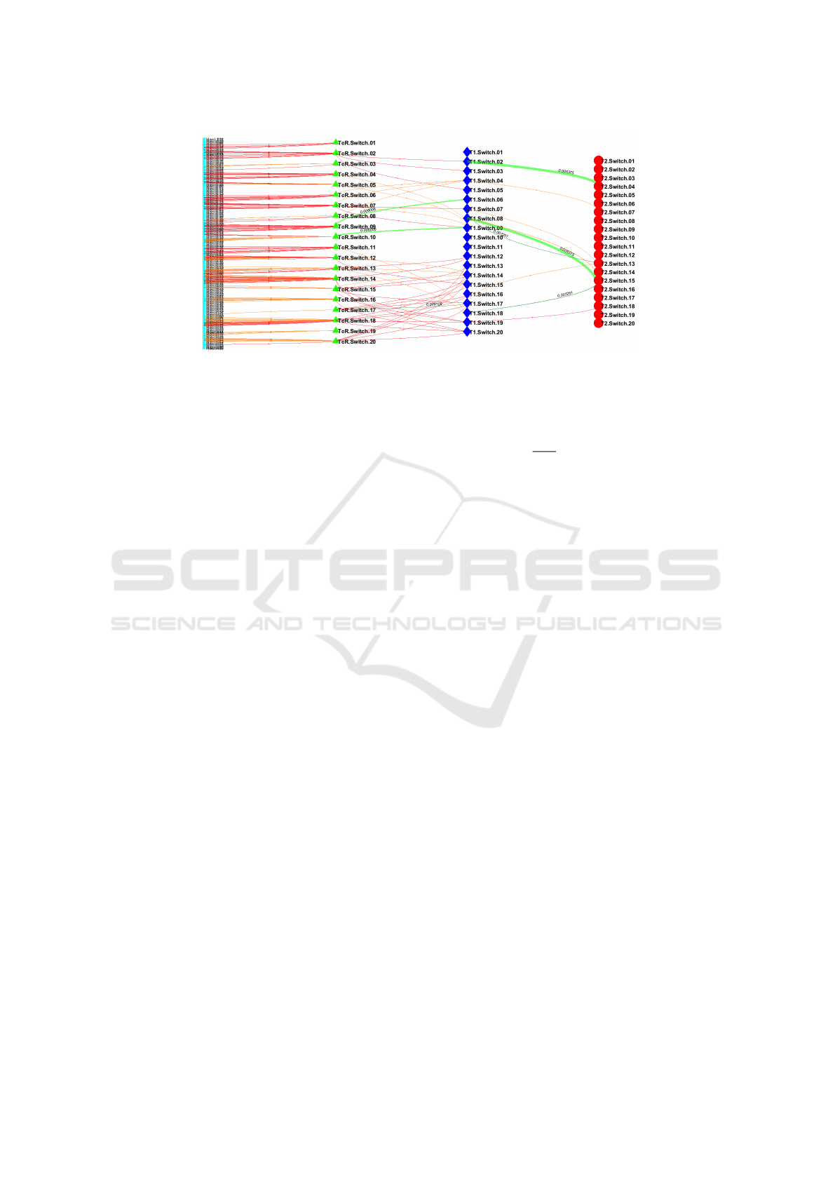
Figure 2: The state of the datacenter described in Section 4.1 at the end of a 30-second simulation. Only the links assigned
a blame score by the 007 diagnostic system (Arzani et al., 2018) are visible here. The thicker the line, the higher the blame
score. The faulty links, totaling seven here, are light green for downlinks and dark green for uplinks. The decimal number on
each is the respective packet-drop probability for that link in the simulation. The healthy links with a blame score are orange
for downlinks and red for uplinks.
the simulator on which they developed the 007 sys-
tem. The datacenters it simulates conform to the Clos
topology. There are four types of machine: a host
machine (Host); a top-of-rack switch (ToR) to which
each Host connects; a further T1 switch to which the
ToRs connect; and a top-level T2 switch. A Pod con-
sists of a set of Hosts, ToRs and T2s. We decided
on 20 T2 switches and two Pods containing 10 T1
switches, 10 Top-of-Rack (ToR) switches and 240
Host devices. Each T1 switch connects to two T2
switches, with each T2 switch connecting to one T1
switch from each Pod. The T1s and ToRs within each
Pod are fully connected to one another. Each ToR
switch connects to 24 Host machines. In total there
are 540 machines or devices and 1440 links, as each
connection consists of an up- and downlink. We use
the blame scores computed by the 007 system in these
simulations to locate faults. Note that faults do not oc-
cur on links joined to Hosts, for detecting such faults
is simple, because they can be detected by the Host
itself directly.
We ran 2,880 30-second simulations of a datacen-
ter randomly selecting 2 to 10 links to be faulty (see
Fig. 2 for an illustration of the topology and an exam-
ple of a simulation). A faulty link is defined as a link
with a packet-drop probability 0.01 ≤ p(F) ≤ 0.1,
while healthy links had a 0% probability of dropping
packets. The dataset is stored on computer as a 2880-
by-1440-by-1 tensor, the one input feature being the
blame scores produced by Arzani et al.’s 007 system.
The labels are stored in a binary 2880-by-1440 tensor,
with faults being the positive class.
Consequent on a low number of failures is a high
class imbalance. The number of faults in a given ex-
periment is uniformly random F ∼ U(2,10), mean-
ing E(F) = 2 +
10−2
2
= 6.5. The expected imbal-
ance ratio is therefore ρ = E(F)/(1440 − E(F)) =
E(F)/E(¬F) = 4.5343 × 10
−3
. Unless this imbal-
ance is addressed, it risks compromising the training,
as the model could reduce the loss simply by labeling
all links healthy.
4.2 Implementation and Comparisons
Our DGCNN consists of three of the directed con-
volutions described in Section 3 and a final 10-unit
multi-layer perceptron (MLP), the output of which is
z = σ(W(c
1
◦ c
2
◦ c
3
)(V, f )+ b), (4)
c
i
(V, f ) = τ(β(g(V, f ))), (5)
where c
i
(V, f ) is the ith convolution block, consist-
ing of a directed convolution g(V, f ) supplied with a
graph structure V and a signal mapping f ; a batch-
normalization layer β and a rectified linear unit τ.
Three of layers are composed (c
1
◦c
2
◦c
3
) and the
output is passed through a sigmoid-activated single-
unit fully connected layer with weights W ∈ R
1×d
and
bias b ∈ R, where d is the number of output maps
from the final convolution block.
Each convolution layer g yields 10 output maps.
The batch-normalization layer uses the default pa-
rameters for Tensorflow (momentum = 0.99,ε =
0.001,β = 0,γ = 1; the moving mean and variance
were zero- and one-initialized respectively). There
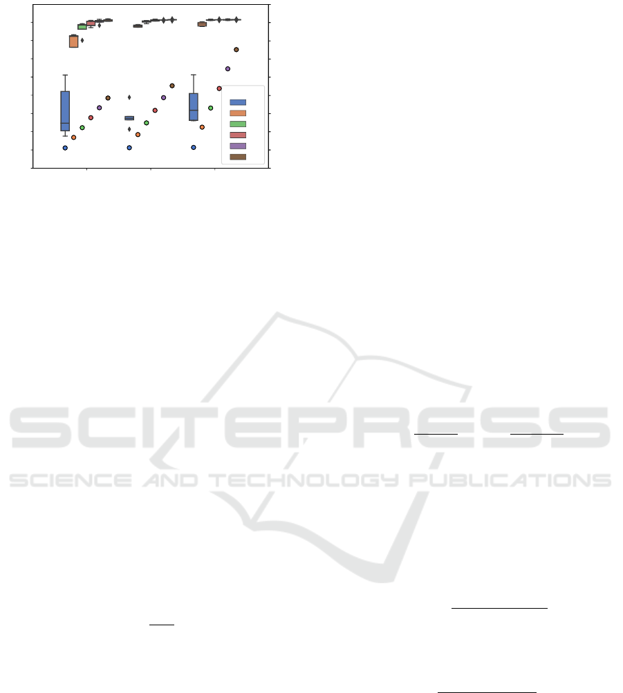
are 731 trainable parameters in total. We decided on 3
convolutional layers and 10 output maps after exper-
imentation, choosing the best trade-off between F
1
-
score and time to train (Fig. 3).
The output z ∈ R
|E|
is the model’s certainty of a
fault at each edge, since the loss is the cross-entropy
Locating Datacenter Link Faults with a Directed Graph Convolutional Neural Network
317
5 10 20
No. Output Maps
0.40
0.45
0.50
0.55
0.60
0.65
0.70
0.75
0.80
F
1
-score
No. Layers
1
2
3
4
5
6
50
100
150
200
250
300
350
400
450
500
Time to train (s)
50
100
150
200
250
300
350
400
450
500
Time to train (s)
Figure 3: The F
1
-score (box plot) and time to train (circles)
for DGCNN networks with varying numbers of convolution
layers and output maps under the experimental conditions
outlined in Section 4.3. Two outliers at five output maps
with 2 layers (0.024429) and 5 layers (0.024123) were ex-
cluded for clarity.
of the output z and the binary vector of edge labels,
where an entry is positive if the corresponding edge is
faulty.
The architecture of the DGCNN differs from the
comparison models only in its convolutional layers g;
we endeavored to keep everything else equal to ensure
that we are assessing a single factor, thereby eliminat-
ing confounding factors. Our comparison models are
the following:
1. Two Undirected Forms of the DGCNN,
(UGCNN and UGCNN Large) to determine the
contribution made to the DGCNN’s performance
by including edge direction. The smaller model
(“undirected graph convolutional neural network
(UGCNN)”) uses 10 output maps per layer, to-
taling 521 parameters The larger one (“UGCNN
large”) uses 12 output maps per layer, totaling
721 parameters, in order to test whether the DGC-
NNs’s greater capacity rather than the inclusion of
edge direction lends it an advantage.
g(x) = θ
0
1
d(x)
∑
y∈Γ(x)
f (y)
+ θ
2
f (x) +b
(6)
2. A GraphSAGE Network (GraphSAGE), to
compare the DGCNN to a similar spatial GCNN.
It is a point of comparison with the wider litera-
ture as a well-cited model. We use the implemen-
tation in version 0.6.0 of the Spektral Tensorflow
library (Grattarola and Alippi, 2020) and the mean
aggregator proposed in the original paper (Hamil-
ton et al., 2017).
3. A Dense Model (Dense), where the convolutional
layers are replaced with 10-unit fully connected
layers, to establish the utility of the structural in-
formation provided by the linegraph.
4.3 Experimental Conditions
The dataset was split 3:1:1 by simulation between
training (1728 simulations), validation (576) and test
set (576) in five folds to study the models’ stability. In
experiments, we chose batches 64 samples large be-
cause it permitted a smooth cosine decay of the learn-
ing rate while keeping the time to train minimal. By
changing the magnitude of the learning rate we found
that a decay from η = 1 × 10
−2
to η = 1 × 10
−7
re-
sulted in the fastest optimization, which occurred by
50 epochs for all models in the experiments. We re-
confirmed these observations by studying the conver-
gences of the F
1
-score on the training and validation
sets over the training period.
The weights of the neural networks’ layers were
initialized using the Glorot uniform initializer, be-
cause they work well with rectified linear units, as
demonstrated in the original paper (Glorot and Ben-
gio, 2010). The biases were initialized at zero, with
the exception of the final fully connected layer, ini-
tialized to a balanced odds-ratio of the positive and
negative samples (7). These same ratios were used
to weight positive and negative links in the loss-
function, the binary cross-entropy of the predictions
and the link labels.
s
−
=
|L(G)|
2 · E(F)
s
+
=
|L(G)|
2 · E(¬F)
(7)
The models are compared on statistics commonly
used in binary problems. Each statistic was computed
on the inferences from the test set and averaged over
the five folds. The primary metric on which we com-
pare the models is the F
1
-score (8). We are however
more interested in precision than recall, as we con-
sider a set of positives as unadulterated by healthy
links to be the ideal situation.
F
1
= 2 +
precision · recall
precision + recall
(8)
We also compare our model’s predictions pairwise
with the other models’ using McNemar’s test (9),
χ
2
=
(|N
s f
− N
f s
| − 1)
2
N
s f
+ N
f s
, (9)
where N
s f
is the count of correct predictions by model
1 where model 2 was incorrect, and N
f s
is the oppo-
site. When χ
2
≈ 0, there is not much difference be-
tween the two models; a large value indicates a differ-
ence in performance. Model 1 in our experiments is
the DGCNN, and model 2 is a comparison models.
We also measure the number of parameters each
model uses, and the average training and inference
times on the test set.
ICPRAM 2021 - 10th International Conference on Pattern Recognition Applications and Methods
318
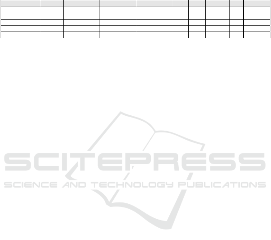
Table 1: The results of the experiments outlined in Sections 4.2 and 4.3. The count of parameters (Params.) is the number of trainable
parameters in the model. The F
1
-score, precision and recall scores are rounded to four decimal places. The results of McNemar’s test (χ
2
)
are rounded to two decimal places. The time to train (“TTT”; in minutes, rounded to nearest second) and inference time (“Inf.”; rounded to
nearest millisecond) are the average times over the five folds.
Model Params. F
1
Precision Recall TTT Inf. N
s f
N
f s
χ
2
DGCNN (ours) 731 .8048 ± .0041 .6736 ± .0056 .9997 ± .0004 2.85 553 — — —
UGCNN large 721 .7657 ± .0161 .6211 ± .0213 .9988 ± .0009 2.30 447 446.6 4.2 432.60
UGCNN small 521 .7312 ± .0688 .5803 ± .0822 .9987 ± .0011 2.27 397 946.0 5.8 927.13
GraphSAGE 311 .3031 ± .0156 .1790 ± .0109 .9924 ±.0030 8.88 4759 14173.6 0.4 14170.40
Dense 311 .3085 ± .0546 .1839 ± .0389 .9893 ± .0072 1.52 219 14245.6 0.4 14242.40
5 RESULTS AND DISCUSSION
As we can see from the results listed in Table 1, the
DGCNN outperformed the comparison models on all
measures. McNemar’s test shows that the DGCNN
frequently classified links correctly where the other
models failed. Our model was also the most stable, as
measured by standard deviation between the folds—
although this could be the consequence of choosing
the architecture, the hyperparameters and experimen-
tal settings on the basis of the performance of the
DGCNN alone.
The number of parameters in the DGCNN slightly
increased the training time over its undirected forms
and nearly doubled it compared to the dense network.
Understandably, inference time on the DGCNN was
middling, having had the greatest number of parame-
ters; for the opposite reason, the dense network is the
fastest. GraphSAGE was exceptionally slow in train-
ing and inference, although this might be owed to this
particular implementation.
The performance of the DGCNN does not appear
to be owed solely to the greater number of parameters:
the evidence is strong that the inclusion of graph di-
rection has helped the DGCNN. The large UGCNN’s
greater capacity improved its performance, but still a
distance off the DGCNN’s performance. As repeated
throughout this paper and elsewhere (Bronstein et al.,
2017), this experiment affords positive evidence that
in knowing the structure we can learn something im-
portant about the signal. We suspect that the mean
aggregator’s unification of a target vertex’s features
with its neighbors’ is deleterious to performance, as
it prevents the model weighting one against the other,
permitting the model to compare a vertex to its neigh-
borhood as our model can.
It is not clear how much performance would be
affected in this particular case if the healthy links
were initialized with small yet insignificant packet-
drop probabilities, as in the original work by Arzani
et al.. It would be interesting to see the effect of the
noise from healthy links on the models’ performance.
For lack of space and time, we also did not conduct
further analyses into the faults that the model missed.
Such analysis could reveal any trends in the types of
the faults not detected.
Having focused on spatial convolutional tech-
niques on graphs in our research, we did not evaluate
the two spectral methods outlined in Section 2 (Ma
et al., 2019; Cui et al., 2020). Our suspicion is that,
being spectral methods, they would not be suitable for
locating multiple independent but related signals on
the graph, as they inherently learn localized but global
signals. We leave this analysis to future work.
6 CONCLUSION
In this paper we presented a spatial convolutional
layer for directed graphs, and moreover a technique
to learn a localization task on a directed linegraph.
We applied these techniques to locating link faults in
a datacenter, finding that the inclusion of direction
found in the graph structure significantly improved
the model. Future work should repeat these experi-
ments, to establish whether similar performance gains
can be yielded in other, unrelated domains, and com-
pare spatial and spectral approaches on other vertex-
focused tasks. This work has focused on simulated
datacenters, because the ground-truths are easily ac-
quired. In further and more specific future work, how-
ever, we could also apply our method to data from
larger, real datacenters.
REFERENCES
Aigner, M. (1967). On the linegraph of a directed graph.
Mathematische Zeitschrift, 102(1):56–61.
Arzani, B., Ciraci, S., Chamon, L., Zhu, Y., Liu, H., Pad-
hye, J., Loo, B. T., and Outhred, G. (2018). 007:
Democratically Finding the Cause of Packet Drops.
In USENIX Symposium on Networked Systems Design
and Implementation, pages 419–435.
Battaglia, P. W., Hamrick, J. B., Bapst, V., et al. (2018).
Locating Datacenter Link Faults with a Directed Graph Convolutional Neural Network
319

Relational inductive biases, deep learning, and graph
networks. ArXiv.
Bronstein, M. M., Bruna, J., Lecun, Y., Szlam, A., and Van-
dergheynst, P. (2017). Geometric Deep Learning: Go-
ing beyond Euclidean data.
Bruna, J., Zaremba, W., Szlam, A., and LeCun, Y. (2014).
Spectral networks and deep locally connected net-
works on graphs. In International Conference on
Learning Representations.
Chen, Z., Bruna, J., and Li, L. (2019). Supervised commu-
nity detection with line graph neural networks. In In-
ternational Conference on Learning Representations.
Cui, J., Zhuang, H., Liu, T., and Wang, H. (2020). Semi-
Supervised Gated Spectral Convolution on a Directed
Signed Network. IEEE Access, 8:49705–49716.
Defferrard, M., Bresson, X., and Vandergheynst, P. (2016).
Convolutional neural networks on graphs with fast lo-
calized spectral filtering. In Advances in Neural Infor-
mation Processing Systems.
Gill, P., Jain, N., and Nagappan, N. (2011). Understand-
ing Network Failures in Data Centers: Measurement,
Analysis, and Implications. ACM SIGCOMM Com-
puter Communication Review, 41(4):350.
Gilmer, J., Schoenholz, S. S., Riley, P. F., Vinyals, O., and
Dahl, G. E. (2017). Neural message passing for quan-
tum chemistry. In International Conference on Ma-
chine Learning, volume 3, pages 2053–2070.
Glorot, X. and Bengio, Y. (2010). Understanding the dif-
ficulty of training deep feedforward neural networks.
In Journal of Machine Learning Research.
Grattarola, D. and Alippi, C. (2020). Graph Neural Net-
works in TensorFlow and Keras with Spektral. ArXiv.
Guo, C., Yuan, L., Xiang, D., et al. (2015). Pingmesh: A
Large-Scale System for Data Center Network Latency
Measurement and Analysis. In SIGCOMM Computer
Communication Review.
Hamilton, W., Ying, Z., and Leskovec, J. (2017). Induc-
tive Representation Learning on Large Graphs. In
Guyon, I., Luxburg, U. V., Bengio, S., Wallach, H.,
Fergus, R., Vishwanathan, S., and Garnett, R., editors,
Advances in Neural Information Processing Systems,
pages 1024–1034. Curran Associates, Inc.
Ji, W., Duan, S., Chen, R., Wang, S., and Ling, Q. (2018).
A CNN-based network failure prediction method with
logs. In Chinese Control And Decision Conference,
pages 4087–4090. IEEE.
Jørgensen, P. B., Jacobsen, K. W., and Schmidt, M. N.
(2018). Neural Message Passing with Edge Updates
for Predicting Properties of Molecules and Materials.
In Conference on Neural Information Processing Sys-
tems.
Kipf, T. N. and Welling, M. (2017). Semi-Supervised Clas-
sification with Graph Convolutional Networks. In In-
ternational Conference on Learning Representations.
Klicpera, J., Groß, J., and G
¨
unnemann, S. (2020). Direc-
tional Message Passing for Molecular Graphs. In-
ternational Conference on Learning Representations,
pages 1–13.
Krzakala, F., Moore, C., Mossel, E., Neeman, J., Sly, A.,
Zdeborov
´
a, L., and Zhang, P. (2013). Spectral re-
demption in clustering sparse networks. Proceedings
of the National Academy of Sciences of the United
States of America, 110(52):20935–20940.
Levie, R., Monti, F., Bresson, X., and Bronstein, M. M.
(2019). CayleyNets: Graph Convolutional Neural
Networks with Complex Rational Spectral Filters.
IEEE Transactions on Signal Processing.
Li, J., Sun, P., and Hu, Y. (2020). Traffic modeling and op-
timization in datacenters with graph neural network.
Computer Networks.
Ma, Y., Hao, J., Yang, Y., Li, H., Jin, J., and Chen, G.
(2019). Spectral-based Graph Convolutional Network
for Directed Graphs. ArXiv.
Monti, F., Boscaini, D., Masci, J., Rodol
`
a, E., Svoboda, J.,
and Bronstein, M. M. (2017). Geometric deep learn-
ing on graphs and manifolds using mixture model
CNNs. In IEEE Conference on Computer Vision and
Pattern Recognition.
Niepert, M., Ahmed, M., Kutzkov, K., Ahmad, M., and
Kutzkov, K. (2016). Learning Convolutional Neural
Networks for Graphs. In International Conference on
Machine Learning, pages 2014–2023.
Protogerou, A., Papadopoulos, S., Drosou, A., Tzovaras,
D., and Refanidis, I. (2020). A graph neural net-
work method for distributed anomaly detection in IoT.
Evolving Systems.
Shuman, D. I., Narang, S. K., Frossard, P., Ortega, A., and
Vandergheynst, P. (2013). The emerging field of signal
processing on graphs: Extending high-dimensional
data analysis to networks and other irregular domains.
IEEE Signal Processing Magazine, 30(3):83–98.
Sperduti, A. and Starita, A. (1997). Supervised neural net-
works for the classification of structures. IEEE Trans-
actions on Neural Networks.
Srinivasan, S. M., Truong-Huu, T., and Gurusamy, M.
(2019). Machine Learning-Based Link Fault Identifi-
cation and Localization in Complex Networks. IEEE
Internet of Things Journal, 6(4):6556–6566.
Wang, M., Cui, Y., Wang, X., Xiao, S., and Jiang, J. (2018).
Machine Learning for Networking: Workflow, Ad-
vances and Opportunities. IEEE Network, 32(2):92–
99.
Xiao, Y., Xing, C., Zhang, T., and Zhao, Z. (2019). An In-
trusion Detection Model Based on Feature Reduction
and Convolutional Neural Networks. IEEE Access,
7:42210–42219.
Zhang, Y., Ge, Z., Greenberg, A., and Roughan, M. (2005).
Network Anomography. In ACM SIGCOMM Confer-
ence on Internet Measurement.
ICPRAM 2021 - 10th International Conference on Pattern Recognition Applications and Methods
320
