
Dynamic Lot Sizing in a Self-organizing Production
Martin Krockert, Marvin Matthes and Torsten Munkelt
Faculty of Computer Science, Dresden University of Applied Sciences, Friedrich-List-Platz 1, Dresden, Germany
Keywords:
Self-organization, Lot Sizing, Group Technology, Job Shop, Setup Time Reduction, Multi-Agent-Systems.
Abstract:
Companies more and more offer individual products to satisfy their customers and stand out from other com-
petitors. Those individual products differ in their production process and thus require many different tool-
resource combinations, so called setups. In order to reduce the number of setups, shortening the overall setup
time, reducing throughput time, while increasing the adherence to delivery dates, we propose a dynamic lot
sizing approach that combines separate operations into so-called buckets. In this paper, we present the im-
plementation of the dynamic lot sizing approach in our multi-agent based self-organizing production, using
two different production models, which demonstrate the efficiency of our solution in comprehension to an
exhaustive rule to create buckets as a results of an empirical study.
1 INTRODUCTION
Today, the increasing needs for companies to offer in-
dividualized products to their customers to stand out
from other competitors, poses new challenges for man
and machine, especially in the area of piece goods
production, where a high degree of product diversifi-
cation leads to the development of ever new tools and
thus to ever new machine tool combinations, so called
setups. The process to equip a tool on a machine takes
time and is referenced as setup time in production
context. Production facilities usually group products
that require the same setup to be produced together as
lots. Under the assumption of producing individual
goods for every customer it is not viable to create lots
based on products, because every product will require
different setups. This will lead to high frequent setup
changes on machines. Irrespective of all measures
to shorten setup times technologically, setup times of
considerable length still occur(Kim and Bobrowski,
1994; M. M. Orta-Lozano and B. Villarreal, 2015).
However, it is still necessary to create lots in order
to reduce frequent setup changes on machines. It is
well known that long setup times extend throughput
times and reduce effective capacity utilization(Spence
and Porteus, 1987). In order to reduce the number
of setups, thereby shortening the overall setup time,
reducing their negative effects, while maintaining a
high adherence to delivery dates as our main goal, we
present a dynamic lot sizing approach, which groups
together operations with the same setup requirements
in so-called buckets. These buckets are only created
temporarily. The operations assigned to the buckets
are processed sequentially by the machine. After a
machine processed an operation the material can be
routed onwards and is not bound to the bucket. In
this way, our dynamic lot sizing approach differs from
conventional lot sizing, which usually keeps lots to-
gether during the processing of their production or-
ders.
The paper is organized as follows: The next sec-
tion classifies the problem and provides a review of
related work. Section III declares the approach in-
cluding components and procedure for dynamically
lot sizing. Subsequently, Sections IV describes our
empirical study. Finally, Section V concludes and
gives an outlook on feature work.
2 PROBLEM DESCRIPTION
2.1 Classification
Customers want more and more individual products.
But no company today can afford to not take these
individual wishes into account. This results in many
different products which can not be produced together
and thus even smaller lots in production. Planing for
individual products makes it very difficult to achieve
a good central production plan. Creating an optimal
schedule for job shop productions is even regarded as
NP-complete (Garey et al., 1976; Domschke et al.,
Krockert, M., Matthes, M. and Munkelt, T.
Dynamic Lot Sizing in a Self-organizing Production.
DOI: 10.5220/0010300803610367
In Proceedings of the 13th International Conference on Agents and Artificial Intelligence (ICAART 2021) - Volume 1, pages 361-367
ISBN: 978-989-758-484-8
Copyright
c
2021 by SCITEPRESS – Science and Technology Publications, Lda. All rights reserved
361

1997; Herrmann, 2011). The problem still remain
NP-complete by integrating setup times (Ng et al.,
2005). In addition, deviations of processing times
and machine failures occur, which invalidate plans
and lead to inefficient production. To counteract these
negative occurrences, we present a method to dynam-
ically create lots in the form of buckets.
Figure 1: Lots;(A) production orders based; (B) operation
based.
According to (Z
¨
apfel, 1982), a lot is defined as
the quantity of a product that passes through the
production process as one item as shown in Fig-
ure 1A. However, this is impossible due to the na-
ture of individual products, where the product struc-
ture and their operations differs, and therefore can
not be combined to lots. The only remaining pos-
sibility is to build lots based on operations of prod-
ucts which require the same machine setups - so
called Group Technologies.(Kusiak, 1987; Gombin-
ski, 1967) Those Group Technologies share the same
technology requirements, but can be assigned to dif-
ferent products(Ham et al., 1985; Brennan, 1995).
Consequently, the operations combined to one
group can be seen as a horizontal cross-linked ag-
gregation of different products over the same Group
Technology (see Figure 1B). By grouping operations
requiring the same technology, the schedule becomes
more efficient, because operations of the same group
can be processed without intermediate machine se-
tups. This directly eliminates additional setup times
compared to pure priority heuristics.
Because of the uncertainty about the product
structures, required machines and required setups of
the newly created product which should satisfy the
customer individual needs, it is not possible to deter-
mine an optimal bucket size for the production objec-
tives. In current manufacturing environments, suffer-
ing from high uncertainty, group heuristic dispatching
rules have become the most common solution (Klaus-
nitzer et al., 2017). Dispatching rules are generally
applied to queues to prioritize the operation to be pro-
cessed next. Those rules mostly aim to reduce setup
times and increase processing efficiency in production
(Frazier, 1996; Ruben et al., 1993; Grabot and Gen-
este, 1994; van der Zee et al., 2011). Several stud-
ies with focus on flow cell manufacturing and group
heuristics already exist (Klausnitzer et al., 2017; Fra-
zier, 1996; Egilmez et al., 2016). There are also pos-
sibilities to solve the scheduling problem using mixed
integer linear programming (MILP) but as it requires
complete and accurate knowledge about all operations
and has high computational cost, even for small prob-
lem sizes, we do not consider MILP.
Group scheduling heuristics can be divided
into two categories - exhaustive and non-
exhaustive(Frazier, 1996). While exhaustive rules
process all operations of the same Group Technology
existing in one queue together, non-exhaustive rules
allow splitting of grouped operations and therefore
switching of setups even though there are still
operations remaining requiring the current setup.
In previous research from Frazier, exhaustive rules
prove to be superior to non-exhaustive rules in flow
shop production (Frazier, 1996). As our research
focuses on high flexibility and robustness in a job
shop production, we developed a non-exhaustive
approach and compare it with an exhaustive heuristic.
Our problem is a job shop scheduling problem
including setup times, which differs from the flow
shop problem analyzed by Frazier. But like Frazier,
we cover uncertainty: Production orders arrive after
exponentially distributed inter-arrival times, and
processing times of operations are log-normally
distributed.
2.2 Disadvantages of Exhaustive Group
Heuristics
To validate that exhaustive heuristics lead to good per-
formance in a highly dynamic production, we created
different test scenarios. Therefore we created two
production models and three setup models, which we
combined to six different scenarios as shown in Table
1. The production is organized as decentralized man-
ufacturing grid, where products can be routed freely
between all machines. Our production model con-
sists of three different machine groups. Machines
can be equipped with different tools. It is possible
to equip multiple machines with a tool of the same
kind at the same time. Working with the same tool
on many machines offers flexibility in production, es-
pecially when the proportion of setups differs and a
single setup potentially dominates.
The size of the production model determines the
amount of machines created for each machine group.
The size of the setup model determines the number
of tools each machine of a machine group can be
equipped with. The product has a three level deep
bill of materials, which consists of 14 materials and
each material requires up to three operations to be
ICAART 2021 - 13th International Conference on Agents and Artificial Intelligence
362

Table 1: Production scenarios.
Production with
number of machines
Setup Model with number of
tools equipable to machines
Scenario
Model
Saw Drill Assembly Size Saw Drill Assembly
1 Small 2 2 2
2 A 2 1 2 Medium 4 4 7
3 Large 8 8 14
4 Small 2 2 2
5 B 4 2 4 Medium 4 4 7
6 Large 8 8 14
produced. Each operation is connected to a previously
defined machine group. During the model creation,
the setups are assigned in a round robin procedure to
each operation, where the assignment is restricted by
the machine group of the operation. For example, an
operation for sawing a wooden panel is assigned to
the machine group ”saws”. While creating the model,
the operation will be assigned to a specific setup i.e.,
”small saw blade”. The setup model size is deter-
mined, based on the number of operations assigned
to setups of a machine group. The lower bound, rep-
resented by the small setup model, uses the minimum
of two setups to ensure at least one setup change. The
large setup model, which represents the upper bound,
uses as many setups as there are operations. That
means all operations’ setups differ from each other.
As medium setup model, we calculated the number
of setups by dividing the numbers of the large setup
model by two. We tested an exhaustive heuristic with
the model combinations from Table 1. The tests show
that using an exhaustive heuristic leads to high setup
times. The tests with large setup models demonstrate,
that in extreme cases, the heuristic leads to a lower
timeliness caused by limitations of production capac-
ities through high setup times, as shown in Table 2.
3 THE DYNAMIC LOT SIZING
APPROACH
3.1 Components of the Approach
The dynamic lot sizing approach is based on three
components: a set of operations, a set of machines,
and a ”bucket manager” for organizing the operations
in buckets.
The first component contains operations from pro-
duction orders. We assume that each production order
consists of a fixed sequence of operations to be pro-
cessed in that sequence. Consequentially, we do not
consider alternative or parallel operations. Each op-
eration contains the following information: estimated
processing duration, due time of the production order,
Table 2: Exhaustive Heuristic KPI.
Production
Model
Setup
Model
Timeliness
Throughput
time in min
Setup
time
Model A
Small 100.0% 274 26.8%
Medium 76.8% 746 31.6%
Large 22.2% 1274 35.6%
Model B
Small 100.0% 277 29.0%
Medium 100.0% 475 39.2%
Large 69.6% 901 44.1%
average duration of the transition between two con-
secutive operations, required setup, and earliest start
as well as latest start obtained by forward and back-
ward scheduling. The second component contains the
machines. Each machine provides a certain capabil-
ity, i.e. drilling capability, and can be equipped with
similar tools, i.e. drills. In order to process oper-
ations, the machine must be equipped with the re-
quired tool, while each tool has a sequence indepen-
dent setup time. Each machine and tool combination
is referenced as setup and is capable to fulfill a certain
capability, i.e. drill a hole with a diameter of one cen-
timeter. However, a machine can only be equipped
with one tool at a time.
The third component is the ”bucket manager”. It
is a persistent instance that organizes buckets and
schedules those buckets on machines. It assigns open
operations requiring the same Group Technology to
buckets linked to the same setup. If there is no suit-
able bucket for an operation, the bucket manager will
create a new bucket and assign the operation to this
bucket. After creating a bucket, the allocation of the
bucket to the machine starts. A separate scheduling
procedure allocates the bucket to the machine. The
procedure can be any scheduling algorithm, while the
bucket manager organizes the buckets, which are cre-
ated upon or filled with incoming operations. To en-
able multiply machines to process buckets requiring
the same setup, multiple buckets can be created. This
way we maintain flexibility by splitting or merging
buckets. Nevertheless, each bucket must contain at
least one operation. This is the operation the bucket
manager originally created the bucket for. After the
creation of the bucket, further operations can be added
depending on the time scope of the bucket. To de-
termine the time scope, we schedule the production
order forwards and backwards when it enters the pro-
duction. In order to guarantee a robust production,
we limit the bucket not only based on the time scope.
We also introduce a method to dynamically limit the
bucket size depending on existing machines and se-
tups for a certain capability. Thus, we ensure that the
production stays flexible and achieves its objectives.
After processing the last operation of the bucket, the
operation is removed from the bucket and the bucket
Dynamic Lot Sizing in a Self-organizing Production
363
dissolves.
3.2 Determine the Bucket Limits
Finding a suitable bucket size is crucial for the dy-
namic lot sizing: Buckets that are too small lead to
more frequent setups, while buckets that are too large
block the machine for too long with one setup, and
thus the production will lose flexibility. The bucket
size determines the operations that fit in a bucket and
will be later on processed sequentially on a machine.
To find a suitable bucket size, we use two mecha-
nisms. Based on the symbol definition in Table 3,
we firstly create a dynamic time scope for the bucket,
limited by subtracting the earliest and latest start time,
obtained from forward and backward scheduling of
the first operation assigned the to bucket (see 1). The
release time of the production order strongly influ-
ences the dynamic time scope, because production or-
ders with a late release lead to small time scopes and
production orders with an early release lead to large
time scopes. Hence, the dynamic time scopes devi-
ate considerably. To avoid too large time scopes, we
implemented a second limitation.
Table 3: Symbol definition.
Symbol Definition
c capability with c ∈ C
s setup s ∈ S
d processing duration d > 0
sbt start time from backward scheduling
s f t start time from forward scheduling with (sbt > s ft)
o is a column vector
with (c, s, d, sbt, s f t)
T
O is a set {o
1
, ··· , o
n
} of operations
S
c
includes all setups assigned
to a capability
M
c
includes all machines assigned
to a capability
f bucket factor with f > 0
w
s
workload with
∑
o∈O
s
o
d
∑
o∈O
c
o
d
l limit with l ≥ 0
The second limitation takes the current number of
machines and their possible setups as well as a bucket
factor into account. The bucket factor is predefined
upon the underlying production and can be experi-
mentally determined. The initial value of the bucket
factor can be based on the length of working shifts,
such as 8, 4 or 2 hours. To verify if an operation fits
into a bucket, we calculate a setup limit by taking the
number of machines and setups of the capability as
well as the current workload of the setup into account
(see 2). This consideration is necessary due to the im-
pact of numbers of machines and numbers of setups
to the bucket size. This means, more possible setups
should lead to larger buckets, while more machines
should lead to smaller buckets. As defined in equa-
tion 3 we determine the bucket minimum by taking
the smaller number from scope limit and setup limit.
l
scope
= sbt
o
1
− s ft
o
1
(1)
l
setup
= f ·
S
c
M
c
· w
s
(2)
l
bucket
= min(l
scope
;l
setup
) (3)
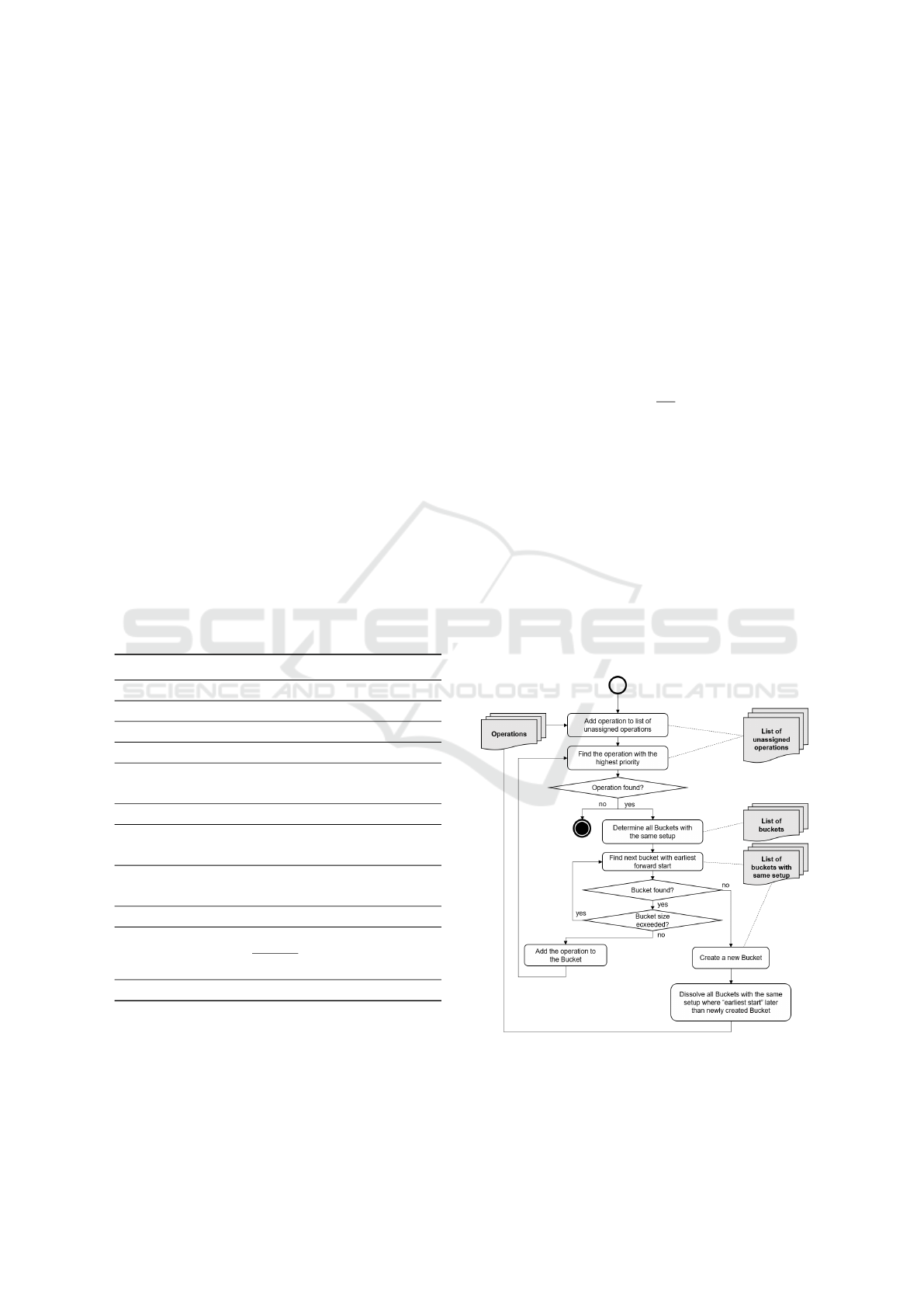
3.3 Procedure to Create, Modify or
Dissolve Buckets
As mentioned before, buckets are virtual elements.
The bucket manager creates, modifies or dissolves
buckets event-based when new operations occur and
have to be assigned to a bucket. At the beginning, all
operations of the production orders are added to the
list of unassigned operations. The procedure (shown
in Figure 2) repeats itself as long as unassigned oper-
ations exits.
Figure 2: Procedure to assign operations to buckets.
Firstly, the procedure selects the operation with
the highest priority from the list of unassigned op-
erations. If any unassigned operation exits, the pro-
ICAART 2021 - 13th International Conference on Agents and Artificial Intelligence
364
cedure selects all buckets from the list of buckets re-
quiring the same setup as the operation. After select-
ing the buckets, the procedure loops through the these
buckets prioritized by the earliest start and calculates
whether the operation fits inside the current bucket or
not. The operation will fit inside this bucket if the
sum of the duration of all the bucket’s operations in-
cluding the new operation is lower or equal than the
dynamically calculated limit of the bucket (see 4).
l
bucket
≤
∑
o∈O
d(o)
+ d
unassigned operation
(4)
If this is the case, the operation will be added to
the bucket. If no suitable bucket can be found or
the bucket size of all found buckets is exceeded, the
bucket manager creates a new bucket, assigns the op-
eration to the bucket and schedules the bucket at any
of the capable machines. After creating a new bucket,
all other buckets with the same setup and an earliest
start later than the earliest start of the newly created
bucket dissolve into their operations. These opera-
tions are rescheduled during the next loop of the pro-
cedure.
3.4 The Bucket Life-cycle
The scheduling mechanism schedules the bucket as
soon as it is created. After assigning a bucket to a
machine, the bucket remains in the planning queue
in front of the machine. The machine picks the next
bucket from the planning queue using the least slack
time (LST) rule. From all due date based rules, LST
is the rule best known for achieving high timeliness
and high throughput (Kannan and Lyman, 1994). Of
course LST can be replaced by any other priority rule,
but this contribution does not consider other rules.
Our approach includes the setup time in the calcula-
tion of the LST. All operations are queued regardless
of whether their preconditions have been met or not.
It is likely that a bucket contains operations that are
not ready to be processed as their materials are not
yet in stock or preceding operations of the same pro-
duction order are not yet completed. Until the bucket
is fixed, new operations can be added and removed
or the bucket can be dissolved. But at some point a
bucket has to be fixed, so that no operation can be
added or removed anymore. In our scenario we fix
the bucket when it is considered to be the next bucket
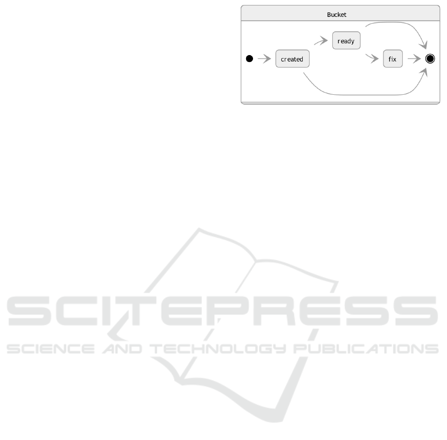
to be processed. We achieve this by giving the bucket
three states. Figure 3 shows all three states of the
bucket and the transitions between them.
If at least one operation of the bucket receives ma-
terial and the preceding operation is completed, we
set the state of the operation and the bucket to ready.
Once setting the bucket ready, we enable the machine
Figure 3: The state transition of a bucket.
to select the bucket from the planning queue in front
of the machine. At this time, new operations can still
be inserted into the bucket. The bucket reaches the
state fix when the machine selects the bucket as the
next bucket to be processed. At that moment, all op-
erations of the bucket without satisfied preconditions
are sent back to the bucket manager and trigger the
procedure in Figure 2 to find or create a new bucket. It
is not possible to insert new operations into the bucket
in state fix. Anyway, it is possible that the bucket will
be dissolved if the bucket is not yet set to fix.
After the machine chooses the bucket and sets its
state to fix, the machine organizes the processing of
the operations of the bucket. In general the operations
in the bucket are unsorted. However, the operations
can be processed according to any priority rule. For
our empirical study we apply the LST.
4 EXPERIMENTAL RESULTS
4.1 General Assumptions
We implemented the dynamic lot sizing approach into
our agent-based simulation of a self-organized pro-
duction (described in detail at (Munkelt and Krockert,
2018)) and compared it with an exhaustive heuristic
based on LST. The exhaustive heuristic processes all
operations of the machine queue sequentially, which
are matching the currently equipped setup and having
all preconditions satisfied. Only after all operations
for the matching setup were processed, the machine
decides for which operation to set-up next, prioritized
by the LST.
For our simulation model, we assume the follow-
ing simulation parameters. In order to test our dy-
namical lot sizing approach, our production runs for
two weeks, 24 hours a day. During this time, we gen-
erate new sales orders for different products with a
product structure list with a maximum depth of three
levels and at least 2 operations per material. During
the simulation of the production, new sales orders ar-
Dynamic Lot Sizing in a Self-organizing Production
365

Table 4: Test scenario for bucket.
Exhaustive Heuristic Dynamic Lot Sizing Differences
Production
Model
Setup
Model
Timeliness
Throughput
time in min
Setup
time
Timeliness
Throughput
time in min
Setup
time
∆ Timeliness
∆ Throughput
time
∆ Setup
time
Model A
Small 100.0% 274 26.8% 95.4% 259 20.8% -4.8% -5.8% -28.8%
Medium 76.8% 746 31.6% 76.8% 610 28.0% ± 0.0% -22.1% -12.9%
Large 22.2% 1274 35.6% 58.9% 772 30.6% +62.4% -61.7% -16.3%
Model B
Small 100.0% 277 29.0% 100.0% 259 19.3% ± 0.0% -6.8% -50.3%
Medium 100.0% 475 39.2% 99.7% 454 28.4% -0.3% -4.6% -38.0%
Large 69.6% 901 44.1% 91,5% 803 29.9% +23.9% -12.2% -47.5%
rive continuously at the production. The inter-arrival
time of customer orders is exponentially distributed as
(Z
¨
apfel and Braune, 2005) and (Ko
ˇ
sturiak and Gre-
gor, 1995) suggest. We choose an inter-arrival time
based on the available capacity to simulate a well uti-
lized production and not cause an overload. There-
fore, new orders arrive approximately every 40 min-
utes at the production model ”A” and every 25 min-
utes at the production model ”B”. To enable one order
overtake another order, the delivery date is evenly dis-
tributed in an interval of 12 hours with an average of
36 hours. To simulate disturbances in the production
process and examine the flexibility of our approach,
we vary the processing times of the operations. The
processing times are distributed log-normally. Trans-
portation times are not considered yet, but can be rep-
resented by an additional operation assigned to the
material. Starting with an empty production, the pro-
duction reaches its steady state after approximately 24
hours in all simulated models. In addition we add an-
other 24 hours before we start the measurement of the
KPIs. For the constant bucket factor we determined
a value of 960 by experiments for all our production
models. Table 5 summarizes the simulation parame-
ters.
4.2 Simulation Results
The simulation results are shown in Table 4 and
demonstrate the superiority of the dynamical lot siz-
ing over the exhaustive heuristic for the empirically
tested production models. The dynamic lot sizing out-
performs the exhaustive heuristic especially when the
production model becomes more complex by consid-
ering more machines and more setups. The timeliness
of the small to medium sized setup models decreases
slightly for the first tested production model, at the
same time the model combination reduces the setup
time by 30%. The setup times in general were re-
duced by 30-50% for all simulated models. The rea-
son is, that the exhaustive heuristic schedules oper-
ations to all machines equally and therefore the ma-
chines permanently switch between various setups. In
contrast, the dynamic lot sizing groups similar oper-
ations and enforces buckets to be processed on one
machine with a suitable setup. Due to the lower setup
time, the machine has more capacity to process opera-
tions. This leads to an increased adherence to delivery
dates indicated by a higher timeliness, while the re-
duced throughput times indicates a more flexible and
robust scheduling.
Table 5: Simulation parameters.
Value Unit Description
14(3) days simulation end time (with settling time)
32 hours release time for production orders
36 hours average time from order placement to delivery
25 minutes average inter-arrival time of new products (Model A)
40 minutes average inter-arrival time of new products (Model B)
20 % deviation of operation’s expected processing time
960 minutes bucket factor to estimate maximum bucket size
5 CONCLUSION
The target of our research was to decrease setup time
in a highly diverse production characterized by un-
certainty. For this purpose, we developed a concept to
non-exhaustively group operations requiring the same
setup. We developed an algorithm for dynamic lot siz-
ing and applied the algorithm to our agent based sim-
ulation using two different production models. Then,
we simulated a two week production cycle and were
able to prove the viability of our approach. In our
simulation model, we were able to reduce throughput
times, the timeliness of sales orders and the average
setup times, while completing the same amount of or-
ders. The results also show that our approach per-
forms excellent with both production models while
we are able to maintain the flexibility and robustness,
although the processing times of the operations devi-
ate. The only trade off is currently, that we have to
experimentally determine the ”bucket factor”. In the
future, we want to investigate further possibilities to
dynamically adapt this factor by taking environmen-
tal conditions into account, i. e. the current workload
ICAART 2021 - 13th International Conference on Agents and Artificial Intelligence
366

of our machines, the average duration of the transi-
tion time for operations of one setup and the times of
releasing buckets into the production. To gain more
general results, we want to investigate further sim-
ulation parameters like different setup distributions,
more divers variants of our production model and dy-
namic generated product structures. We are also look-
ing forward to apply our approach to real world sce-
narios of the companies we are cooperating with.
ACKNOWLEDGEMENTS
The authors acknowledge the financial support by
the German Federal Ministry of Education and Re-
search within the funding program ”Forschung an
Fachhochschulen” (contract number: 13FH133PX8).
REFERENCES
Brennan, R. W. (1995). Modeling and analysis of manufac-
turing systems. isbn 0-417-51418-7 [pp.461]. Inter-
national Journal of Computer Integrated Manufactur-
ing, 8(2):155–156.
Domschke, W., Scholl, A., and Voß, S. (1997). Produc-
tion planning: aspects of industrial engineering (Pro-
duktionsplanung: Ablauforganisatorische Aspekte).
Springer-Lehrbuch. Springer, Berlin, 2.,
¨
uberarb. und
erw. aufl. edition.
Egilmez, G., Mese, E. M., Erenay, B., and S
¨
uer, G. A.
(2016). Group scheduling in a cellular manufactur-
ing shop to minimise total tardiness and nt: a compar-
ative genetic algorithm and mathematical modelling
approach. International Journal of Services and Op-
erations Management, 24(1):125.
Frazier, G. V. (1996). An evaluation of group scheduling
heuristics in a flow-line manufacturing cell. Inter-
national Journal of Production Research, 34(4):959–
976.
Garey, M. R., Johnson, D. S., and Sethi, R. (1976).
The complexity of flowshop and jobshop scheduling.
Mathematics of Operations Research, 1(2):117–129.
Gombinski, J. (1967). Group technology - an introduction.
Production Engineer, 46(9):557–564.
Grabot, B. and Geneste, L. (1994). Dispatching rules in
scheduling: a fuzzy approach. International Journal
of Production Research, 32(4):903–915.
Ham, I., Hitomi, K., and Yoshida, T. (1985). Group technol-
ogy: Applications to production management. Inter-
national series in management science/operations re-
search. Kluwer-Nijhoff, Boston.
Herrmann, F. (2011). Operational planning in IT systems
for production planning and control: (Operative Pla-
nung in IT-Systemen f
¨
ur die Produktionsplanung und
-steuerung). Vieweg+Teubner, Wiesbaden.
Kannan, V. R. and Lyman, S. B. (1994). Impact of family-
based scheduling on transfer batches in a job shop
manufacturing cell. International Journal of Produc-
tion Research, 32(12):2777–2794.
Kim, S. C. and Bobrowski, P. M. (1994). Impact of
sequence-dependent setup time on job shop schedul-
ing performance. International Journal of Production
Research, 32(7):1503–1520.
Klausnitzer, A., Neufeld, J. S., and Buscher, U. (2017).
Scheduling dynamic job shop manufacturing cells
with family setup times: a simulation study. U. Lo-
gist. Res.
Ko
ˇ
sturiak, J. and Gregor, M., editors (1995). Simulation of
production systems (Simulation von Produktionssyste-
men). Springer Vienna, Vienna.
Kusiak, A. (1987). The generalized group technology con-
cept. International Journal of Production Research,
25(4):561–569.
M. M. Orta-Lozano and B. Villarreal (2015). Achieving
competitiveness through setup time reduction. In 2015
International Conference on Industrial Engineering
and Operations Management (IEOM), pages 1–7.
Munkelt, T. and Krockert, M. (2018). Agent-based self-
organization versus central production planning. In
2018 Winter Simulation Conference (WSC), pages
3241–3251, [Piscataway, NJ]. IEEE.
Ng, C. T., Cheng, T. C. E., Janiak, A., and Kovalyov, M. Y.
(2005). Group scheduling with controllable setup and
processing times: Minimizing total weighted comple-
tion time. Annals of Operations Research, 133(1-
4):163–174.
Ruben, R. A., Mosier, C. T., and Mahmoodi, F. (1993). A
comprehensive analysis of group scheduling heuris-
tics in a job shop cell. International Journal of Pro-
duction Research, 31(6):1343–1369.
Spence, A. M. and Porteus, E. L. (1987). Setup reduction
and increased effective capacity. Management Sci-
ence, 33(10):1291–1301.
van der Zee, D.-J., Gaalman, G. J., and Nomden, G.
(2011). Family based dispatching in manufacturing
networks. International Journal of Production Re-
search, 49(23):7059–7084.
Z
¨
apfel, G. (1982). Production management (Produk-
tionswirtschaft). De-Gruyter-Lehrbuch. de Gruyter,
Berlin.
Z
¨
apfel, G. and Braune, R. (2005). Modern heuristics of pro-
duction planning: (Moderne Heuristiken der Produk-
tionsplanung). WiSo-Kurzlehrb
¨
ucher Reihe Betrieb-
swirtschaft. Vahlen, Munich.
Dynamic Lot Sizing in a Self-organizing Production
367
