ML-based Decision Support for CSP Modelling with Regular
Membership and Table Constraints
Sven L
¨
offler, Ilja Becker and Petra Hofstedt
Department of Mathematics and Computer Science, MINT, Brandenburg University of Technology Cottbus-Senftenberg,
Programming Languages and Compiler Construction Group, Konrad-Wachsmann-Allee 5, 03044 Cottbus, Germany
Keywords:
Constraint Programming, CSP, Refinement, Optimizations, Regular Membership Constraint, Table Constraint,
ML, Machine Learning.
Abstract:
The regular membership and the table constraints are very powerful constraints which allow it to substitute
every other constraint in a constraint satisfaction problem. Both constraints can be used very flexible in a huge
amount of problems. The main question we want to answer with this paper is, when is it faster to use the
regular membership constraint, and when the table constraint. We use a machine learning approach for such
a prediction based on propagation times. As learning input it takes randomly generated constraint problems,
each containing exactly one table resp. one regular membership constraint. The evaluation of the resulting
decision tool with specific but randomly generated CSPs shows the usefulness of our approach.
1 INTRODUCTION
Since the search space of constraint satisfaction prob-
lems (CSPs) is very big and the solution process of-
ten needs an extremely high amount of time we are
always interested in a speed-up of the solution pro-
cess. There are various ways to describe a CSP in
practice and consequently, the problem can be mod-
eled by different combinations of constraints, which
results in the differences in resolution speed and be-
havior.
The regular membership and the table constraints
are both very powerful constraints which allow it to
substitute every other constraint in a constraint satis-
faction problem. Both constraints can be used very
flexible in many problems. In this paper we try to
answer the question whether a regular or a table con-
straint is more suitable in a given CSP, based on ma-
chine learning.
For our test series we create random CSPs with
only one constraint in two different ways with the
expectation, that the CSPs created by one way are
faster solvable with table constraints, and the others
are faster solvable with the regular constraint. Finally,
we evaluate our approach with another random set of
CSPs and give an outlook of our aims for the future.
In this paper we will use the notion of a ”regular
constraint” synonymously for ”regular membership
constraint” or ”regular language membership con-
straint”.
2 PRELIMINARIES
In this section, we introduce necessary definitions
and methods of constraint programming for our
machine learning approach. We consider CSPs which
are defined in the following way:
CSP. A constraint satisfaction problem (CSP) is
defined as a 3-tuple P = (X ,D,C) where X =
{x
1
,x
2
,...,x
n
} is a set of variables, D = {D
1
,D
2
,...,
D
n
} is a set of finite domains such that D
i
is the do-
main of x
i
, and C = {c
1
,c
2
,...,c
m
} is a set of con-
straints.
Constraint. A constraint c
j
= (X
j
,R
j
) ∈ C is a rela-
tion R
j
, which is defined over the variables X
j
⊆ X of
the constraint c
j
(Dechter, 2003).
Next, we define the two essential constraints for this
work, the regular constraint and the table constraint.
For the definition of the regular constraint we first
need the definition of a deterministic finite automaton
(DFA).
Deterministic Finite Automaton. A deterministic fi-
nite automaton M is a five tuple (Q, Σ, δ, q
0
, F),
where:
974
Löffler, S., Becker, I. and Hofstedt, P.
ML-based Decision Support for CSP Modelling with Regular Membership and Table Constraints.
DOI: 10.5220/0010299109740981
In Proceedings of the 13th International Conference on Agents and Artificial Intelligence (ICAART 2021) - Volume 2, pages 974-981
ISBN: 978-989-758-484-8
Copyright
c
 2021 by SCITEPRESS – Science and Technology Publications, Lda. All rights reserved

• Q is a finite set of states,
• Σ is a finite alphabet,
• δ is a transition function Q × Σ → Q,
• q
0
∈ Q is a initial state,
• and F ⊆ Q is a set of final states.
A word (w
1
w
2
...w
n
) = w ∈ Σ
∗
is accepted by an au-
tomaton M iff w is element of the language, which is
described by the automaton: w ∈ L(M).
In this paper, the considered automatons have a
certain structure: The set of states Q can be be parti-
tioned into Q = Q
0
∪ ... ∪ Q
n+1
, such that transitions
are only possible form a state of level Q
i
to a state
of level Q
i+1
. Furthermore, Q
0
contains only the ini-
tial state q
0
and Q
n+1
contains only the singleton final
state q
f inal
.
Maximum Width. The maximum width of such an au-
tomaton M corresponds to the maximum number of
states in one level:
maxWidth(M) = max(|Q
i
| ∀i ∈ {0,...,n}). (1)
Regular Constraint. The regular constraint guar-
antees for a DFA M = (Q,Σ,δ,q
0
,F) and an or-
dered set of variables {x
1
,...,x
n
} = X
0
∈ X with
domains {D
1
,...,D
n
} = D
0
⊆ D, where D
i
⊆
Σ | ∀i ∈ {1,...,n}, that for each variable assignment
φ
j
(x
1
,...,x
n
) = (d
j,1
,...,d
j,n
) the word d
j,1
...d
j,n
is ac-
cepted by the automaton M (van Hoeve and Katriel,
2006).
regular({x
1
,...,x
n
},M) = {(w
1
,...,w
n
) | ∀i ∈
{1,...,n},where w
i
∈ D
i
, (w
1
.. . w
n
) ∈ L(M)}.
(2)
The table constraint is an intensively researched con-
straint (Bessi
`
ere and R
´
egin, 1997; Lecoutre, 2011;
Lecoutre et al., 2015; Lecoutre and Szymanek, 2006;
Lhomme and R
´
egin, 2005; Mairy et al., 2014).
Table Constraint. A positive (resp. a negative) ta-
ble constraint guarantees for an ordered set of vari-
ables {x
1
,..., x
n
} = X
0
∈ X and a list of tuples T ,
that for each variable assignment φ
j
(x
1
,..., x
n
) =
(d
j,1
,..., d
j,n
) the tuple t
j
= (d
j,1
,..., d
j,n
) must (not)
be element of the tuple list T . For all positive table
constraints follows accordingly:
table({x
1
,..., x
n
},T ) := {(d
j,1
,..., d
j,n
) ∈ T
| ∀ j ∈ {1,..., |T |}}.
(3)
For a speed comparison of two constraints c
1
and c
2
,
we must guarantee that both are equivalent. Thus,
we define that two constraints c
1
= (X
1
,R
1
) and c
2
=
(X
2
,R
2
) are equivalent, if they cover the same vari-
ables X
1
b=X
2
and describe the same tuples with their
relations R
1
and R
2
.
Furthermore, two propagators p
1
and p
2
are equiva-
lent if they correspond to equivalent constraints and
propagate the same value eliminations for equal do-
mains resp. domain changes.
2.1 A Regular and a Table Propagator
Both the regular and the table constraint can repre-
sent every other constraint and they both reach the
same consistency level: Generalized Arc Consistency
(GAC)
1
. Thus, they are suitable as competitors for
each other.
We use the regular propagator introduced by
Gilles Pesant in (Pesant, 2004), for further details we
refer to the original source.
The table constraint is implemented by different
propagators across different solvers but also within
the same solver. For example the Choco Solver
(Prud’homme et al., 2017) alone has more than ten
different propagators for the table constraint. It fol-
lows a list of acronyms, under which the algorithms
are known in literature:
• AC2001, AC3, AC3rm, AC3bit+rm, CT, FC,
GAC2001, GAC2001+, GAC3rm, GAC3rm+,
GACSTR+, MDD+, and STR2+.
The Compact Table algorithm (CT) was chosen here
because it is very effective and amongst others default
in the Choco Solver (for positive tuple sets with more
than 500 tuples), in Oscar (OscaR, 2018) and in the
Google OR Tools (LLC, 2019).
The CT algorithm was introduced in (Demeule-
naere et al., 2016) and will only be mentioned here.
For a description and details we suggest the original
source.
Since the regular propagator and the CT propaga-
tor both reach GAC, and they correspond to equiv-
alent constraints (regular and table constraint), they
are also equivalent.
3 COMPACTNESS OF REGULAR
CONSTRAINTS
The Hypotheses 1 and 2 (see below) for our machine
learning approach suggest that the ratio of the num-
ber of tuples |T | of a table constraint c
t
= (X,T ) by
the number of transitions |M.∆| resp. the width of the
corresponding automaton M of an equivalent regular
constraint c
r
= (X,M) can be indicators for the con-
straint type which solves the problem faster. We call
1
At least the two propagators we use for our approach.
ML-based Decision Support for CSP Modelling with Regular Membership and Table Constraints
975

q
0,0
start
M
1
=
q
1,0
1,2,3
q
2,0
1,2,3
q
3,0
1,2,3
x
1
x
2
x
3
T
1
= {{1, 1,1},{1, 1,2}, {1,1, 3},{1,2, 1},{1, 2,2},
{1,2, 3},{1, 3,1}, {1,3,2}, {1,3, 3},{2,1, 1},
{2,1, 2},{2, 1,3}, {2,2,1}, {2,2, 2},{2,2, 3},
{2,3, 1},{2, 3,2}, {2,3,3}.{3, 1,1}, {3,1,2},
{3,1, 3},{3, 2,1}, {3,2,2}, {3,2, 3},{3,3, 1},
{3,3, 2},{3, 3,3}}
Figure 1: The tuple set T
1
and the automaton M
1
for
two equivalent constraints c
1
t
= (x
1
,x
2
,x
3
,T ) and c
1
r
=
(x
1
,x
2
,x
3
,M), with a compact automaton M.
this ratios CiT (compactness in transitions) resp. CiW
(compactness in width):
CiT = |T |/|M.∆|, (4)
CiW = |T |/width(M). (5)
Hypothesis 1. Given a regular constraint c
r
= (X ,M)
and an equivalent positive table constraint c
t
= (X ,T ).
If the CiT value for these constraints exceeds a certain
threshold, then using the regular constraint c
r
is more
promising than the table constraint c
t
, and otherwise
vice versa.
Hypothesis 2. Given a regular constraint c
r
=
(X,M) and an equivalent positive table constraint c
t
=
(X,T ). If the CiW value for these constraints exceeds
a certain threshold, then using the regular constraint
c
r
is more promising than the table constraint c
t
, and
otherwise vice versa.
Both hypotheses are motivated by the fact that for
finding one solution a table constraint has to unselect
all tuples but one via the supports and the regular con-
straint has to remove all transitions of all paths from
the initial state to the final state of the automaton but
one (if using the mentioned propagators).
The Figures 1 and 2 show the automatons M
1
and
M
2
of regular constraints c
1
r
and c
2
r
, and the tuples T
1
and T
2
of equivalent table constraints c
1
t
and c
2
t
. The
constraints c
1
r
and c
1
t
represented in Figure 1 allow all
possible combinations of the values 1, 2, and 3 for
the variables x
1
,x
2
, and x
3
, whereas, the constraints
c
2
r
and c
2
t
shown in Figure 2 allow all possible combi-
nations of the values 1, 2, and 3 for the variables x
1
,x
2
and x
3
, where the sum of the variables x
1
,x
2
and x
3
is
equal to a variable x
4
∈ {3,...,9}.
In both cases, there are 27 solutions, but in the
first case it’s a very compact automaton (with only 9
transitions) and in the second case a bigger automaton
(with 34 transitions). So in case one, six transitions
must be removed for the instantiation of a solution,
while in case two this are 30 transitions. In each case,
26 supports (representing the tuples) must be removed
in the corresponding table constraint.
q
0,0
start
M
2
=
q
1,1
1
q
1,2
2
q
1,3
3
q
2,4
3
2
1
q
2,2
1
q
2,3
2
1
q
2,5
3
2
q
2,6
3
q
3,6
3
2
1
q
3,3
1
q
3,4
2
1
q
3,5
3
2
1
q
3,9
3
q
3,8
3
2
q
3,7
3
2
1
q
4,0
3
4
5
6
7
8
9
x
1
x
2
x
3
x
4
T
2
= {{1, 1,1,3}, {1,1, 2,4},{1, 2,1, 4},{2,1, 1,4},
{1,1, 3,5}, {1,2,2, 5},{1, 3,1,5}, {2,1, 2,5},
{2,2, 1,5}, {3,1,1, 5},{1, 2,3,6}, {1,3, 2,6},
{2,1, 3,6}, {2,2,2, 6},{2, 3,1,6}, {3,1, 2,6},
{3,2, 1,6}, {1,3,3, 7},{2, 2,3,7}, {2,3, 2,7},
{3,1, 3,7}, {3,2,2, 7},{3, 3,1,7}, {2,3, 3,8},
{3,2, 3,8}, {3,3,2, 8},{3, 3,3,9}}
Figure 2: The tuple set T
2
and the automaton M
2
for
two equivalent constraints c
2
t
= (x
1
,x
2
,x
3
,x
4
,T ) and c
2
r
=
(x
1
,x
2
,x
3
,x
4
,M), with a big automaton M.
Because of the different values for CiT
1
= 27/9 vs.
CiT
2
= 27/34 and CiW
1
= 27/1 vs. CiW
2
= 27/7, CiT
and CiW both beeing bigger for the first problem, both
hypothesis suggest that in the first case, the regular
constraint and in the second case the table constraint
propagates relatively faster.
4 GENERATION OF RANDOM
PROBLEM INSTANCES
In this section, we explain the generation of the train-
ing data for the machine learning approach.
The main idea is to generate CSPs P
all
= {P
t
∪
P
r
∪ P
t∗
∪ P
r∗
}, which contain only one table (P
t
) or
regular (P
r
) constraint, and then to create an equiva-
lent CSP P
r∗
i
∈ P
r∗
for each CSP P
t
i
∈ P
t
, which uses
a regular constraint instead of a table constraint, and
vice versa. All other settings, like search strategies,
propagation order etc. are identical for P
t
i
∈ P
t
and
P
r∗
i
∈ P
r∗
(P
r
j
∈ P
r
and P
t∗
j
∈ P
t∗
resp.), so that the time
difference in the solution process should result exclu-
sively from the propagation time of the chosen con-
straint. Thus, the real impact of the used constraints
can be checked. In the following, we explain how we
create our random CSPs in P
t
and P
r
, to guarantee the
quality and transparency of our data.
2
2
The source code used to generate the samples can
be found at: https://git.informatik.tu-cottbus.de/loeffsve/
ICAART 2021 - 13th International Conference on Agents and Artificial Intelligence
976

Table 1: The parameters for the generation of CSPs.
Parameter Range of values
Number of solutions {1,2, ..., 25000}
Number of variables {2,3, ..., 21}
Domain Base {2,3, ..., 200}
∆ domain size {0, 1, ...,
domainSizeBase-1}
Ratio of leaks 0-95%
Maximum width {1,2,...,50}
The CSPs in P
t
are created fully randomly, such that
the solutions of such a CSP P
t
i
∈ P
t
(resp. P
r∗
i
∈ P
r∗
)
are also completely random (e.g. in number and dis-
tribution). In contrast to this, the CSPs in P
r
(resp.
P
t∗
) are created in a way, such that the used automa-
ton M
i
of each CSP P
r
i
∈ P
r
can be represented very
compactly (width(M) ≤ 50).
According to our hypothesis introduced in Section
3, we expect that the CSPs originally created with a
regular constraint can be solved faster faster in its reg-
ular version, and the CPS originally created with a
table constraint can be solved faster with a table con-
straint on average. Furthermore, we hope to find more
accurate hypotheses for the prediction of usefulness
of table and regular constraints.
To have a meaningful data set we created 1000
CSPs originally with table constraints and 1000 CSPs
originally with regular constraints.
For the generation, solving, and learning we
used a computer with a 6 core CPU, 12 threads, at
2.40GHz, with 32 GB RAM memory (2667 MHz),
running the Canonical Ubuntu OS in version 18.04.1.
The algorithms are implemented in Java under JDK
version 1.8.0 231.
For the randomization, we used the Random class
of the java.util package, which uses a 48-bit seed,
which is modified using a linear congruential formula,
as explained in (Knuth, 1997, Section 3.2.1.). As the
initial seed for the problem generation the problem
number (1 to 1000) was used. We used the randomly
instantiated parameters for the problem generation as
presented in Table 1 (in case of table generation the
maxWidth parameter was not used).
The number of solutions is also the number of tu-
ples in the table constraint and also the number of
paths from the initial state to the final state in the
automaton of the corresponding regular constraint.
The domainSizeBase is a base value and the actual
domain size of each variable is calculated based on
domainSizeBase plus or minus a random value be-
tween 0 and the ∆DomainSize value.
The ratio of leaks is the average of the number of
code-generation-table-vs-regular.
domain values |D
i
| divided by the range size of the
domain max(D
i
) − min(D
i
) + 1 for all domains D
i
∈
D.
The following subsections explain the creation of
the CSPs in P
t
and P
r
.
4.1 Table based Problem Instances
Algorithm 1 shows the interaction of the parameters
for the creation of the variables, or more precisely,
for the creation of the domains of the variables. Each
entry values[i] represents the domain D
i
. The algo-
rithm follows exactly the description of the parame-
ters. Each domain size is in an ∆DomainSize (∆DS)
range around the domainSizeBase (dB) (Line 3) and
the possibility for leaks is equal to r (Line 5 to 7). Af-
ter the generation of the variables with Algorithm 1,
nbTuples different tuples will be generated randomly
based on the generated values.
Algorithm 1: createVariables.
Data: int: nbVars, dB, ∆DS
double: r
Result: int[][]: values
1 int[][] values = new int[nbVars]
2 forall (int i = 0; i < nbVars; i++) do
3 values[i] = randomInt(−∆DS,∆DS) + dB
4 forall (int idx = 0,v = 0;
idx < values[i].length; v++) do
5 if (randomDouble() > r) then
6 values[i][idx] = v
7 idx++
8 return values
4.2 Regular based Problem Instances
For the regular based CSP generation the solutions
are not directly generated, rather the automaton M is
generated and subsequently checked, to whether the
number of paths from the initial state to the final state
(so the number of solutions) is in an acceptable range.
The maxWidth parameter limits the maximum width
of the automaton and guarantees that M is compact.
Algorithm 2 shows the generation of automatons
for the CSPs P
r
. The algorithm takes the domains
D = {D
1
,..., D
n
}, the number of variables nbVars and
the maximum width of the automaton maxWidth as
input and returns the states of the created automaton
in a two dimensional array q, where each sub-array
q[i] corresponds to the states Q
i
of level i.
First, the variables are instantiated: The value
lNS, standing for the number of states of the last level,
ML-based Decision Support for CSP Modelling with Regular Membership and Table Constraints
977

Algorithm 2: createAutomaton.
Data: Domains D = {D
1
,..., D
n
}
int nb
Vars
, maxWidth
Result: Node[][] q
1 repeat
2 int lNS = 1
3 int[] nb
Trans
= new int[nb
Vars
]
4 Node[][] q = new Node[nb
Vars
+ 1][]
5 q[0][0] = createFirstState()
6 q[n][0] = createFinalState()
7 forall (int i = 1; i < nb
Vars
; i++) do
8 int cNS = randomInt(1,min(lNS ∗
|D
i−1
|,maxWidth))
9 q[i] = createStates(cNS,i)
10 lNS = cNS
11 nb
Trans
[i − 1] =
randomInt(1, min(lNS ∗
|D
i−1
|,100))
12 nb
Trans
[nb
Vars
− 1] =
randomInt(1, min(lNS ∗
|D
nb
Vars
−1
|,100))
13 addTransitions(nb
Trans
,D)
14 if (maxWidth > 5) then
15 maxWidth − −
16 until checkNbTuples(q);
17 return q
is instantiated with value 1. This represents that at
level 0 is only one state (q
0,0
, Line 2). Each entry
of the integer array nbTrans represents the number of
transitions from level i to level i +1 (Line 3). The two
dimensional node array q will contain the states of
the automaton and is consequently instantiated with
length n + 1 (Line 4).
For each level i ∈ {1 to nbVars}, a random number
of states is created and added to the states array (Lines
8 and 9). The number of states for each level is always
between one and the minimum of the maxWidth value
and the number of states from the last level (lNS) mul-
tiplied by the domain size of the corresponding vari-
able (|D
level−1
|), because this is the maximum number
of states a deterministic automaton (like we use) can
reach in a level.
Afterwards, a random number between one and
100 (resp. the maximum number) is generated, which
represents the number of transitions from level i − 1
to level i (Lines 11 and 12). The bounds maxWidth
and 100 guarantee that the automaton will not be too
big.
The addTransitions method then adds the previ-
ously generated number of transitions to each level
(Line 13) and removes all states which are not part of
at least one path from the initial state to the current
resp. the final state.
The checkNbTuples method counts all paths from
the initial state to the final state, which corresponds
to the number of solutions resp. the number of tuples
of an equivalent table constraint and returns true if
the number of solutions is neither too big nor to small
(Line 16). A new automaton will be generated ran-
domly until the number of solutions is acceptable. In
most cases the automaton will have too many solu-
tions and not few. To reduce the number of solutions,
we reduce the maximum width step by step down to a
minimum of five (Lines 14 and 15).
The bounds, which limit the width of the automa-
ton and the number of transitions lead to the point that
automaton generated in this way is more compact than
automatons, which are created from randomly gener-
ated tuples. Consequently, we expect that the CSPs in
P
r
propagate faster with the regular constraint and the
CSPs in P
t
propagate faster with the table constraint,
on average.
5 MACHINE LEARNING FOR
DECISION MAKING
In the following, we briefly outline the creation of
classifiers with standard machine learning techniques
in our approach.
5.1 Methodology
In order to create learning data we solved each prob-
lem instance, both from our tuple based, as well as au-
tomaton based instances, with both types constraints
(table and regular). For each run we calculated and
stored the problem features, propagator state features,
and the run times. This provides a set of samples of
the following form:
(id, used constraint, ( f
1
,. . ., f
n
),(r
1
,. . .,r
m
)),
where f
i
is a recorded feature as described in Sec-
tion 5.2, r
j
is a recorded result (e.g., run time in ns),
used constraint ∈ {table,regular}, and id being a tu-
ple:
(seed for problem generation,modelling base),
modelling base ∈ {tuple based,automaton based}.
Since the samples represent the following Carte-
sian product:
{modelling base} × {used constr.} × n (= 1000)
we end up with a dataset of 4000 run samples (P
all
).
ICAART 2021 - 13th International Conference on Agents and Artificial Intelligence
978

Since each problem id is run twice, with either a tabu-
lar (P
t
i
,P
t∗
j
) or regular constraint (P
r∗
i
,P
r
j
), this reduces
to 2000 actual problem samples (1000 for each mod-
elling base). For each problem id we then calculate a
number of features, such as the speedup of the faster
vs. the slower constraint, and which constraint was
the fastest. For these we also deduce the classes we
want to predict based upon this data. As of now we
try to classify samples where the speedup was bigger
than 1.5 according to the faster constraint (“regular”,
“table”). The rest we try to identify as “irrelevant”.
The goal of this distinction is to avoid unnecessary
transformations when applying this to real problems.
We furthermore prepare the data by standardizing
the features using the Scikit-Learn StandardScaler.
We then compose tables suitable for machine learning
resulting in samples of the form:
(id, ( f
1
,. . ., f
n
),class ∈ {irrel, regular, table}),
with f
i
being the inputs for our ML approach, and
class being the label the classifier is supposed to pre-
dict.
In the next step, we separate a random subset of
30% of the original data set (by id) for testing. The
remaining 70% are used for training. This results in
a training set of 1400 samples and a testing set of
600 samples. From here we utilise machine learn-
ing to train a classifier. We use the Scikit-Learn li-
brary for easy-to-use, reliable, and proven machine
learning (Pedregosa et al., 2011). From the vast selec-
tion of models available in Scikit-Learn we chose the
Random Forest Classifier (RFC) for this experiment.
RFCs were introduced by (Breiman, 2001), but in-
stead of letting each decision tree vote on the class the
scikit-learn implementation averages the probabilistic
prediction of each tree in the ensemble (scikit-learn
developers, 2020). RFCs tend to deliver reasonably
good results with little hyperparameter optimization
(Hastie et al., 2009, p. 587 ff.). The RFC is configured
with the default parameters provided by Scikit-Learn
in version 0.23.
5.2 Problem Features
We collect a set of measurements from the CSP we
aim to make a decision for. In total we collect 11 fea-
tures which are easy to calculate and which we sus-
pect to possibly be indicators of the CSPs suitability
for one constraint or the other.
Problem Features. Features inherent to the prob-
lem:
• Variable and solution tuple count;
• Minimal, maximum, and average domain size,
domain size delta;
• Average number of leaks and avg. rate of leaks;
• Minimal, maximum, and average domain offset
to zero.
Propagator Features. Features taken from the prop-
agators internal state:
• Number of zeros and ones in supports for table
constraint (cf. (Demeulenaere et al., 2016));
• CiT and CiW, Number of states, edges, and
width, minimal, maximum and avg. branching
degree with respect to the internal DFA, as well
as the number of supports for the regular con-
straint.
5.3 Evaluation of the Problem Instances
We evaluated the classifiers against the previously
separated testing subset, which consists of 291 table,
220 regular and 89 irrel samples. To evaluate the
classifiers against the testing data we trained the clas-
sifiers on the training data and then apply it to the
test data. We trained multiple classifiers on differ-
ent subsets of features. The first subset only contains
problem features. The second subset also includes
the propagator features. In an application scenario
this would require to first instantiate both propagators,
however this can be done efficiently. We then calcu-
lated the following metrics based on the predictions
and correct classification data:
Precision. The precision is the ratio of true positives
to the total number of positively predicted sam-
ples. It encodes how well the classifier differen-
tiates the respective label against other labels. A
high precision on regular and tabular labels is de-
sirable, in order not to actively transform a model
using a slower constraint.
Recall (Sensitivity). The recall value is the ratio of
true positives to the total number of positives. It
encodes how sensitive the classifier is in picking
up on a certain label. Of special interest is the
recall on the regular and tabular label, as these
encode the sensitivity to improvement. However
sensitivity is less important than precision, as it’s
better to miss some improvements than to actively
worsen a model.
F1-Score. The F1-Score encodes a weighted average
of precision and recall. It is calculated as follows:
F1 = 2∗(precision∗recall)/(precision+recall).
For all metrics holds that 1 is the best value and 0 the
worst. The evaluation results for all tested classifiers
are displayed in Table 2 and in the confusion matrices
in Figure 3. Table 2 displays the calculated metrics as
ML-based Decision Support for CSP Modelling with Regular Membership and Table Constraints
979

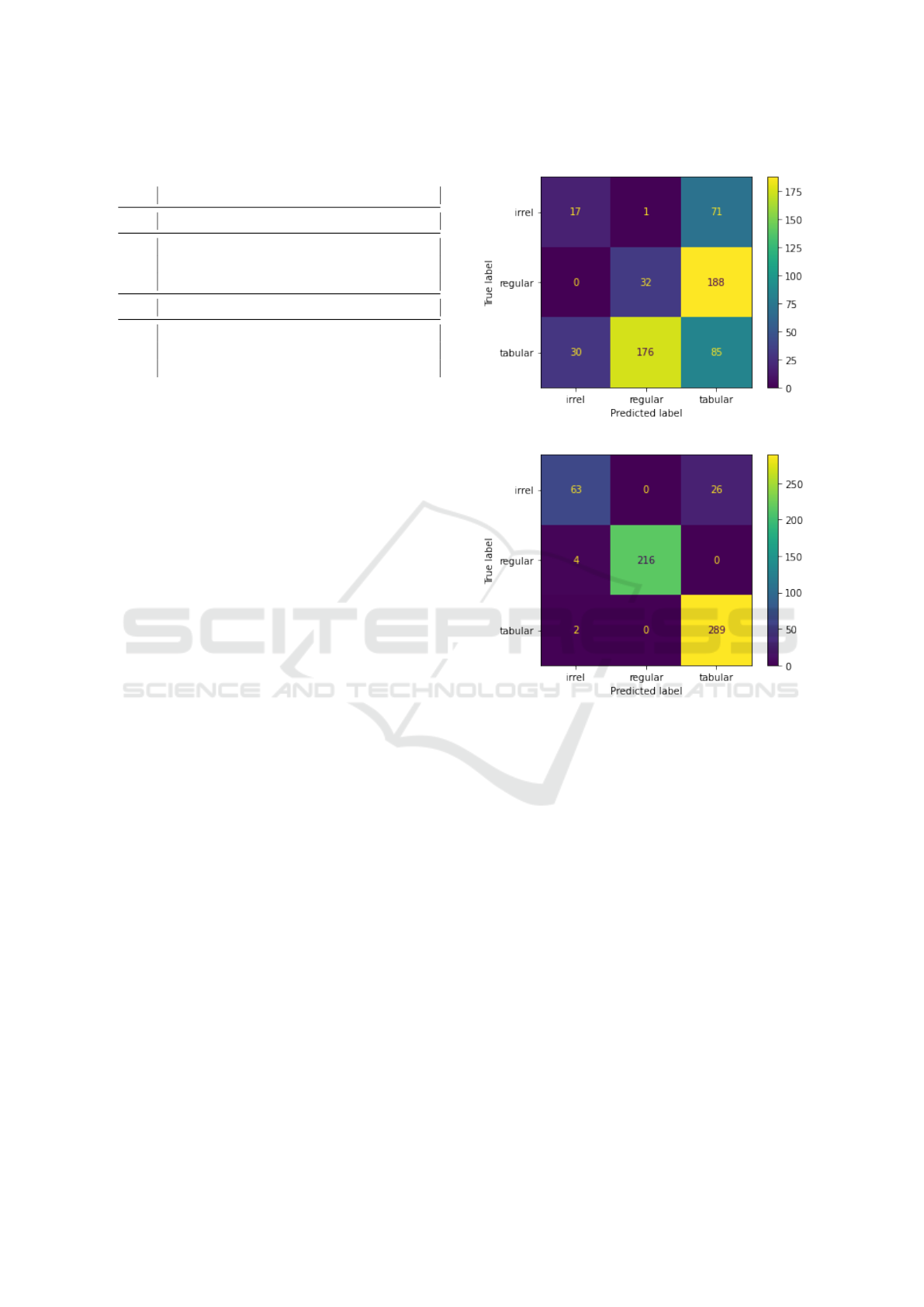
Table 2: Classification metrics of different classifiers tested
against the test data set.
Precision Recall F1-Score Support
Problem Features Only
Irrel. 19.10% 36.17% 25.00% 47
Reg. 14.55% 15.31% 14.92% 209
Tab. 29.21% 24.71% 26.77% 344
Problem and Propagator Features
Irrel. 70.79% 91.30% 79.75% 69
Reg. 98.18% 100.0% 99.08% 216
Tab. 99.31% 91.75% 95.38% 315
well as the number of instances classified correspond-
ingly (support). Figure 3 visualizes how the classifi-
cations are distributed. Ideally all fields are zero but
the top-left to bottom-right diagonal. For the classifier
based on problem features only there are many mis-
classfied cases, especially between tabular and regu-
lar instances. These misclassifications between regu-
lar and tabular are especially undesirable, as they ac-
tively worsen a model. In the matrix for the classifier
that includes propagator features we see that there are
isolated cases of regular and tabular labels misclassi-
fied as irrelevant (left column) and a number of irrel-
evant instances classified as tabular (top-right field).
Two things become evident when looking at the
data: First, while the classifier trained on problem
features only does not perform well at all, the clas-
sifier that also learns on propagator features performs
much better. Second, it appears feasable to predict the
better peforming constraint from features extractable
from the problem and propagators built to represent it.
While the classification is not perfect yet, it does gen-
eralize well from the training data onto the test data
set. Furthermore, the biggest classification inaccura-
cies occur with the irrelevant class, which naturally
does not result in much lost time but the one spent on
classification.
The classification takes less than two milliseconds
(1.17ms on average). Our generated problems have
a median run time of 3.25ms, while the fastest mod-
els have a median run time of 2.21ms. This also does
not include the feature calculation time, so upon first
glance the classification time appears not worth the
trade off. However the classification needs to happen
only once for a constraint within a real problem and
only depends on the RFCs tree depth and count and
therefore should scale well across bigger problems.
We also believe that for a real problem with larger run
times the repeated propagation effort results in a well
scaling speedup, with the increasing absolute savings
making the classification time irrelevant.
Problem Features Only
Problem and Propagator Features
Figure 3: Confusion Matrices over the Classification of the
Generated Test Problems.
The Random Forest Classifier (RFC) implemented in
Scikit-Learn allows a closer look at the importance of
features within the decision trees. While these values
are to be taken with a grain of salt (see (scikit-learn
developers, 2020)), the forests appear to put high im-
portance on the features of the regular constraint (es-
pecially CiT and CiW) and table constraint, as well as
the number of variables, supporting the initially stated
hypotheses.
In conclusion we proved that it is possible to pre-
dict with some certainty whether the tabular or regu-
lar constraint will propagate faster based on problem
features extracted before attempting to solve the prob-
lem. We suspect that these predictions generalize to
constraints embedded in real problems and allow to
reduce their runtimes.
ICAART 2021 - 13th International Conference on Agents and Artificial Intelligence
980

6 CONCLUSION AND FUTURE
WORK
We showed that an ML based approach can be used to
predict whether a regular or a table constraint works
faster in a CSP with a single constraint. A test bench
with 2000 sample CSPs was generated and tested.
Based on these results a classifier was trained which
managed to distinguish models that profit from one or
the other constraint with reasonable precision.
The next step based upon the insights learned with
these experiments is to examine, whether the predic-
tions can help speed up solving real problems. Of
further interest would be, whether and how the fea-
tures extracted from the generated problems differ to
the ones obtained from subsets of real problems. We
would also like to explore further optimizations in the
machine learning approach, as well as the possibility
of deducing rule-based predictive models from the in-
sights gained from the machine learning experiments.
REFERENCES
Bessi
`
ere, C. and R
´
egin, J. (1997). Arc consistency for gen-
eral constraint networks: Preliminary results. In Fif-
teenth International Joint Conference on Artificial In-
telligence, IJCAI 97, 2 Volumes, pages 398–404. Mor-
gan Kaufmann.
Breiman, L. (2001). Random forests. Machine Learning,
45(1):5–32.
Dechter, R. (2003). Constraint processing. Elsevier Morgan
Kaufmann.
Demeulenaere, J., Hartert, R., Lecoutre, C., Perez, G., Per-
ron, L., R
´
egin, J., and Schaus, P. (2016). Compact-
table: Efficiently filtering table constraints with re-
versible sparse bit-sets. In Rueher, M., editor, Princi-
ples and Practice of Constraint Programming - 22nd
International Conference, CP 2016, volume 9892 of
Lecture Notes in Computer Science, pages 207–223.
Springer.
Hastie, T., Tibshirani, R., and Friedman, J. H. (2009). The
Elements of Statistical Learning: Data Mining, Infer-
ence, and Prediction, 2nd Edition. Springer Series in
Statistics. Springer.
Knuth, D. E. (1997). The Art of Computer Programming,
Volume 2: Seminumerical Algorithms. Addison-
Wesley, Boston, third edition.
Lecoutre, C. (2011). STR2: optimized simple tabular re-
duction for table constraints. Constraints An Interna-
tional Journal, 16(4):341–371.
Lecoutre, C., Likitvivatanavong, C., and Yap, R. H. C.
(2015). STR3: A path-optimal filtering algorithm for
table constraints. Artif. Intell., 220:1–27.
Lecoutre, C. and Szymanek, R. (2006). Generalized arc
consistency for positive table constraints. In Ben-
hamou, F., editor, Principles and Practice of Con-
straint Programming - 12th International Conference,
CP, volume 4204 of Lecture Notes in Computer Sci-
ence, pages 284–298. Springer.
Lhomme, O. and R
´
egin, J. (2005). A fast arc consistency
algorithm for n-ary constraints. In Veloso, M. M.
and Kambhampati, S., editors, The Twentieth Na-
tional Conference on Artificial Intelligence and the
Seventeenth Innovative Applications of Artificial In-
telligence Conference, pages 405–410. AAAI Press /
The MIT Press.
LLC, G. (2019). Google LLC, Google OR-Tools, 2019.
Mairy, J., Hentenryck, P. V., and Deville, Y. (2014). Optimal
and efficient filtering algorithms for table constraints.
Constraints An International Journal, 19(1):77–120.
OscaR (2018). OscaR: Operational research in scala. https:
//bitbucket.org/oscarlib/oscar. last visited 2019-08-22.
Pedregosa, F., Varoquaux, G., Gramfort, A., Michel, V.,
Thirion, B., Grisel, O., Blondel, M., Prettenhofer, P.,
Weiss, R., Dubourg, V., VanderPlas, J., Passos, A.,
Cournapeau, D., Brucher, M., Perrot, M., and Duch-
esnay, E. (2011). Scikit-learn: Machine learning in
python. J. Mach. Learn. Res., 12:2825–2830.
Pesant, G. (2004). A regular language membership con-
straint for finite sequences of variables. In Wallace,
M., editor, Principles and Practice of Constraint Pro-
gramming - CP, 10th International Conference, vol-
ume 3258 of Lecture Notes in Computer Science,
pages 482–495. Springer.
Prud’homme, C., Fages, J.-G., and Lorca, X. (2017). Choco
documentation.
scikit-learn developers (2020). scikit-learn user guide, Re-
lease 0.23.2 edition.
van Hoeve, W.-J. and Katriel, I. (2006). Global Constraints.
Elsevier, Amsterdam, First edition. Chapter 6.
ML-based Decision Support for CSP Modelling with Regular Membership and Table Constraints
981