
Reconstruction of Convex Polytope Compositions from 3D Point-clouds
Markus Friedrich
1
and Pierre-Alain Fayolle
2
1
Institute for Computer Science, LMU Munich, Oettingenstraße 67, Munich, Germany
2
The University of Aizu, Ikki machi, Aizu-Wakamatsu, Japan
Keywords:
3D Reconstruction, Geometry Processing, Spatial Clustering, Evolutionary Algorithms.
Abstract:
Reconstructing a composition (union) of convex polytopes that perfectly fits the corresponding input point-
cloud is a hard optimization problem with interesting applications in reverse engineering and rigid body dy-
namics simulations. We propose a pipeline that first extracts a set of planes, then partitions the input point-
cloud into weakly convex clusters and finally generates a set of convex polytopes as the intersection of fitted
planes for each partition. Finding the best-fitting convex polytopes is formulated as a combinatorial optimiza-
tion problem over the set of fitted planes and is solved using an Evolutionary Algorithm. For convex clustering,
we employ two different methods and detail their strengths and weaknesses in a thorough evaluation based on
multiple input data-sets.
1 INTRODUCTION
This work deals with the problem of reconstructing
a solid object from an input 3D point-cloud, where
the solid object is represented as a collection (union)
of convex polytopes (represented as an intersection of
planar half-spaces). We are dealing with the partic-
ular case where the input 3D point-cloud describes a
single, or a few, at most, objects. Larger scenes, made
of multiple objects, can be first decomposed by clas-
sification or semantic segmentation.
Potential applications can be found in reverse en-
gineering, or reconstruction, of buildings from 3D
point-clouds, see for example (Musialski et al., 2013)
or in the field of numerical physics simulations, such
as in the simulation of rigid body dynamics, see for
example (Coumans and Bai, 2019), where the con-
vex decomposition of a solid can increase efficiency,
since the collision of convex bodies can be efficiently
determined (Gilbert et al., 1988).
The problem of reconstructing a set of convex
polytopes from a 3D point-cloud is difficult to solve
since it heavily relies on the robust detection and exact
fitting of planes in the unstructured input point-cloud,
and on finding a correct mapping of these planes in a
set of convex polytopes. The latter is a difficult com-
binatorial problem since neither the number of result-
ing convex polytopes nor the sets of planes that form
particular polytopes are known in advance. Our ap-
proach relies on a pre-segmentation step performed
by a deep neural network, followed by fitting planes
using a RANSAC-based model fitter. Then, a cluster-
ing of the input point-cloud into weakly convex parts
is conducted and the clusters are used by an Evo-
lutionary Algorithm to form a collection of convex
polytopes. Our main contributions are:
• A detailed description and evaluation of a full
pipeline for the detection and fitting of convex
polytopes in an unstructured 3D point-cloud.
• A detailed comparison of clustering methods to
group points in (weakly) convex clusters.
• An efficient Evolutionary Algorithm (EA) to form
a collection of convex polytopes from clusters of
points.
The rest of this paper is organized as follows: First
we discuss works related to our approach in Section 2,
followed by an introduction of the basic concepts used
in the rest of the paper in Section 3. In Section 4,
we describe our reconstruction pipeline in detail. It
is followed by its evaluation in Section 5. Finally, the
paper ends with a brief conclusion and a discussion of
potential future directions of work (Section 6).
2 RELATED WORKS
The problems of segmentation, primitive detection
and fitting are well studied in computer graphics,
computer vision, computer aided design and related
Friedrich, M. and Fayolle, P.
Reconstruction of Convex Polytope Compositions from 3D Point-clouds.
DOI: 10.5220/0010297100750084
In Proceedings of the 16th International Joint Conference on Computer Vision, Imaging and Computer Graphics Theory and Applications (VISIGRAPP 2021) - Volume 1: GRAPP, pages
75-84
ISBN: 978-989-758-488-6
Copyright
c
2021 by SCITEPRESS – Science and Technology Publications, Lda. All rights reserved
75

engineering domains, see for example this survey on
primitive detection (Kaiser et al., 2019) and the refer-
ences therein. We deal in this work with the problem
of reconstructing a solid from a 3D point-cloud as a
composition (union) of convex polytopes. Thus, we
are interested in related works considering problems
such as: plane detection and fitting, cuboid or gen-
eral polytope detection and fitting, among others. In
the following, we list the works most relevant to these
problems.
Segmentation, primitive detection and fitting are
necessary steps in the field of reverse engineering 3D
data, which is the process of recovering a computer
model of a 3D shape from acquired data. See, for ex-
ample, (V
´
arady et al., 1998; Benk
´
o and V
´
arady, 2004)
and the references therein. Approaches in reverse en-
gineering are, however, not limited to the fitting of
planar patches, but deal also with higher order patches
common in industrial design. On the other hand, fitted
planar patches do not have to be arranged into col-
lections of cuboids or convex polytopes in these ap-
proaches unlike the problem that we are dealing with.
A popular technique for fitting models to data (in-
cluding noisy data) is RANSAC (Fischler and Bolles,
1981), as well as its numerous variants. The effi-
cient RANSAC method introduced in (Schnabel et al.,
2007) is a fast RANSAC-based approach for detect-
ing and fitting primitives of different types (plane,
cylinder, sphere, cone) in a 3D point-cloud. The ap-
proach was further improved in (Li et al., 2011) by
enforcing additional constraints during the fitting pro-
cess, such as the fact that two planes are parallel or
perpendicular. The addition of these constraints al-
low for a more robust fitting of the primitives at the
cost of a less efficient approach. While the efficient
RANSAC approach (Schnabel et al., 2007) deals with
unbounded primitives (plane, infinite cylinder), the
method described in (Friedrich et al., 2020) uses addi-
tional steps to generate solid primitives. Our approach
also uses RANSAC as one of its steps. However,
we apply RANSAC to a pre-clustered point cloud,
which allows us to make the process more robust and
less parameter sensitive. In addition, unlike (Schn-
abel et al., 2007) that fits infinite planes, we gener-
ate convex polytopes by combining the initially fit-
ted planes. Note that our approach deals with general
convex polytopes unlike (Friedrich et al., 2020) that
is limited to cuboids.
The efficient detection and fitting of planes in 3D
point-clouds is a necessary step for the reconstruc-
tion of buildings. See for example (Monszpart et al.,
2015; Oesau et al., 2016) and the references therein.
These planes can then be combined to form cuboids
(Xiao and Furukawa, 2014; Li et al., 2016) or more
complex polyhedral shapes (Nan and Wonka, 2017).
In the work (Xiao and Furukawa, 2014), the authors
propose a method to reconstruct museums by fitting
cuboids to the input data and by combining them us-
ing a CSG (Constructive Solid Geometry) expression.
The method described in (Li et al., 2016) assumes
that all fitted planes are perpendicular to one of the
three dominant directions. This allows to recast the
combinatorial problem of combining planes to form
cuboids into an energy minimization problem that can
be solved using graph-cut optimization. Unlike these
works, we deal with the problem of forming a min-
imal (or at least as small as possible) set of general
convex polytopes describing the solid, and are not
limited to cuboids. The method presented in (Nan
and Wonka, 2017) relaxes the constraint that planes
need to be perpendicular to the three main directions
of the data, and instead deals with the minimization of
a binary linear problem that is solved with an off-the-
shelf solver. This approach forms one polytope (not
necessarily convex) for a given input point-cloud. On
the other hand, we deal with the problem of finding
a set of convex polytopes describing the input point-
cloud.
In recent years, techniques from machine learn-
ing, such as deep neural networks, have become pop-
ular tools for problems of classification, segmentation
or fitting/discovery of models from 3D point-clouds.
The approach described in (Tulsiani et al., 2017) uses
a deep neural network to approximate an input 3D
shape by predicting a collection of cuboids.
A method for learning a convex shape decomposition
from an input image, called CvxNet, is introduced in
(Deng et al., 2019). The method consists of train-
ing a deep neural network that defines a solid ob-
ject as a union of convex shapes, where each convex
shape is represented by a combination of planar half-
spaces. The input is assumed to be an image (RGB or
depth image), while we work with unstructured point-
clouds. Furthermore, they assume a fixed number of
polytopes (i.e. their network always output the same
number of convex polytopes).
A related approach for learning a BSP tree (Binary
Space Partition) from an input image or an input voxel
is proposed in (Chen et al., 2019). Similar to our ap-
proach it outputs a collection of convex polytopes de-
scribing an object. However, the approach is based on
learning from a collection of shapes belonging to a set
of categories and is thus restricted to process objects
belonging to these same categories.
GRAPP 2021 - 16th International Conference on Computer Graphics Theory and Applications
76
3 BACKGROUND
3.1 Evolutionary Algorithms
Evolutionary Algorithms are population-based, iter-
ative meta heuristics for solving mainly combinato-
rial optimization problems. The optimization pro-
cess starts with the creation of a population of ran-
domly generated solution candidates. All candidates
in the population are then ranked based on a objec-
tive (or fitness) function which is the formal descrip-
tion of the objective that should be optimized for.
Based on the ranking, a subset of high-ranked solu-
tion candidates are selected to form the next itera-
tion’s population. The rest of the population is filled
with stochastic variations of selected individuals from
the old population. These variations are described in
form of so-called mutation and crossover operators
and are highly domain-specific. Whereas mutation
operators usually alter a single individual randomly,
crossover operators exchange random parts between
two or more individuals. Variation operators are ap-
plied with a certain probability (also called mutation
rate and crossover rate). The execution ends if a cer-
tain termination criteria is met (e.g. maximum num-
ber of iterations or a target quality has been reached).
The main advantage of Evolutionary Algorithms is
their flexibility: Solution candidate representation,
objective function as well as variation operators can
be tailored to specific application domains. Further-
more, the objective function does not have to be dif-
ferentiable like in gradient-based optimization algo-
rithms.
3.2 Convex Polytopes
A 3D convex polytope (in the following convex poly-
tope or polytope w.l.o.g.) is a special-case of a poly-
hedron with the additional property that its surface en-
closes a convex subset of the Euclidean space. A con-
vex polytope can either be described by the intersec-
tion of a set of planar half-spaces (H-representation)
or by its extreme points (V-representation) which are
essentially the vertices of its hull. Our approach forms
convex polytopes out of planes (H-representation) but
also needs the V-representation for volume discretiza-
tion (see Section 4.4.2). The transformation between
H- and V- representation can be done using the Dou-
ble Description method (Fukuda and Prodon, 1996).
In addition, the signed distance from a 3D point x
to the surface of the convex polytope is needed (see
Equation 8) which is
d(x) = min({dot(p
n
, p
o
−x) : (p
o
, p
n
) ∈ P}), (1)
where P is the set of planes forming the convex poly-
tope, p
n
is a plane’s normalized normal, p
o
an arbi-
trary point on the plane and dot(·,·) is the scalar prod-
uct of two 3D vectors.
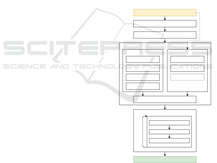
4 PIPELINE
The polytope reconstruction pipeline consists of mul-
tiple steps as depicted in Fig. 1. It starts with a 3D
point-cloud as input and ends with the resulting set
of convex polytopes as output. First, planes are fit-
ted to the input point-cloud (Section 4.1). Then the
point-cloud is structured in order to produce a plane-
neighborhood graph (Section 4.2). The point-cloud is
then clustered in weakly convex parts (Section 4.3).
Finally, an Evolutionary Algorithm is run on each
cluster and its corresponding planes to form a set of
convex polytopes (Section 4.4.2).
Weakly Convex Clustering
Line-Of-Sight
Polytope Generation
Affinity Matrix Computation
Spectral Clustering
Cluster Number Estimation
EA
For each cluster
Polytopes
WCSEG
Polytope Filtering
OR
Proportional Resampling
Point-cloud
Point-cloud Structuring
Plane Extraction
Target Volume Creation
Structured Point-cloud Assignment
Over-Segmentation
Neighbor Patch Merging
Volumetric Merging
Figure 1: The proposed polytope reconstruction pipeline.
4.1 Plane Extraction
In the first step, planes are fitted to the input point-
cloud. We use a clustered variant of the efficient
Reconstruction of Convex Polytope Compositions from 3D Point-clouds
77
RANSAC approach (Schnabel et al., 2007) as de-
scribed in (Friedrich et al., 2020). It starts with a per-
point prediction of primitive types using a deep neural
network which was trained with focus on noise and
outlier robustness. This is followed by a DBSCAN
clustering (Ester et al., 1996) based on the point coor-
dinate, normal and primitive type. Finally, parameters
are extracted using RANSAC for each cluster and the
resulting primitives are merged. The additional clus-
tering provably increases fitting robustness (Friedrich
et al., 2020). This step results in a set of planes P and
a mapping f that associates each plane with a subset
of surface points from O, f
p
: P → P (O), where P is
the power set operator. The result of this step on some
test models is illustrated in Fig. 6b, where points are
colored based on the fitted plane they belong to.
4.2 Point-cloud Structuring
We apply a point structuring mechanism to the in-
put point-cloud O as proposed in (Lafarge and Alliez,
2013). First, points are projected within a given ε on
an occupancy grid located on the surface of their cor-
responding plane (the grid cell size is
√
2ε). The oc-
cupied cell centers are added to the result point set O
s
and marked as points of type ’planar’. Then, the plane
neighborhood graph G
N
= (P,N) is extracted, with
planes P as vertices and edges N whenever two planes
are neighbors (or adjacent). Two planes are consid-
ered to be adjacent if at least two points of each plane
share an edge in the k nearest neighbor (k-NN) graph
of the input point-cloud O. Based on G
N
, creases and
corner points are extracted, and creases are uniformly
sampled using a sampling distance of 2ε. Finally, cor-
ner and sampled crease points are added to O
s
(see
Fig. 6c for labeled result point sets). Please note, that
we are only interested here in the plane neighborhood
graph G
N
and the structured point set O
s
, but not in
the point labeling (’planar’, ’crease’ or ’corner’). O
s
is furthermore free of noise and outliers.
4.3 Weakly Convex Clustering
For point-cloud decomposition in convex or almost
(weakly) convex clusters, we have experimented with
two methods with different performances. Both ap-
proaches result in a set of clusters C with each cluster
c ∈ C containing an associated point-cloud O
c
and a
set of associated planes P
c
.
The results obtained from these weak clustering ap-
proaches on some of our test models are shown in
Fig. 4.
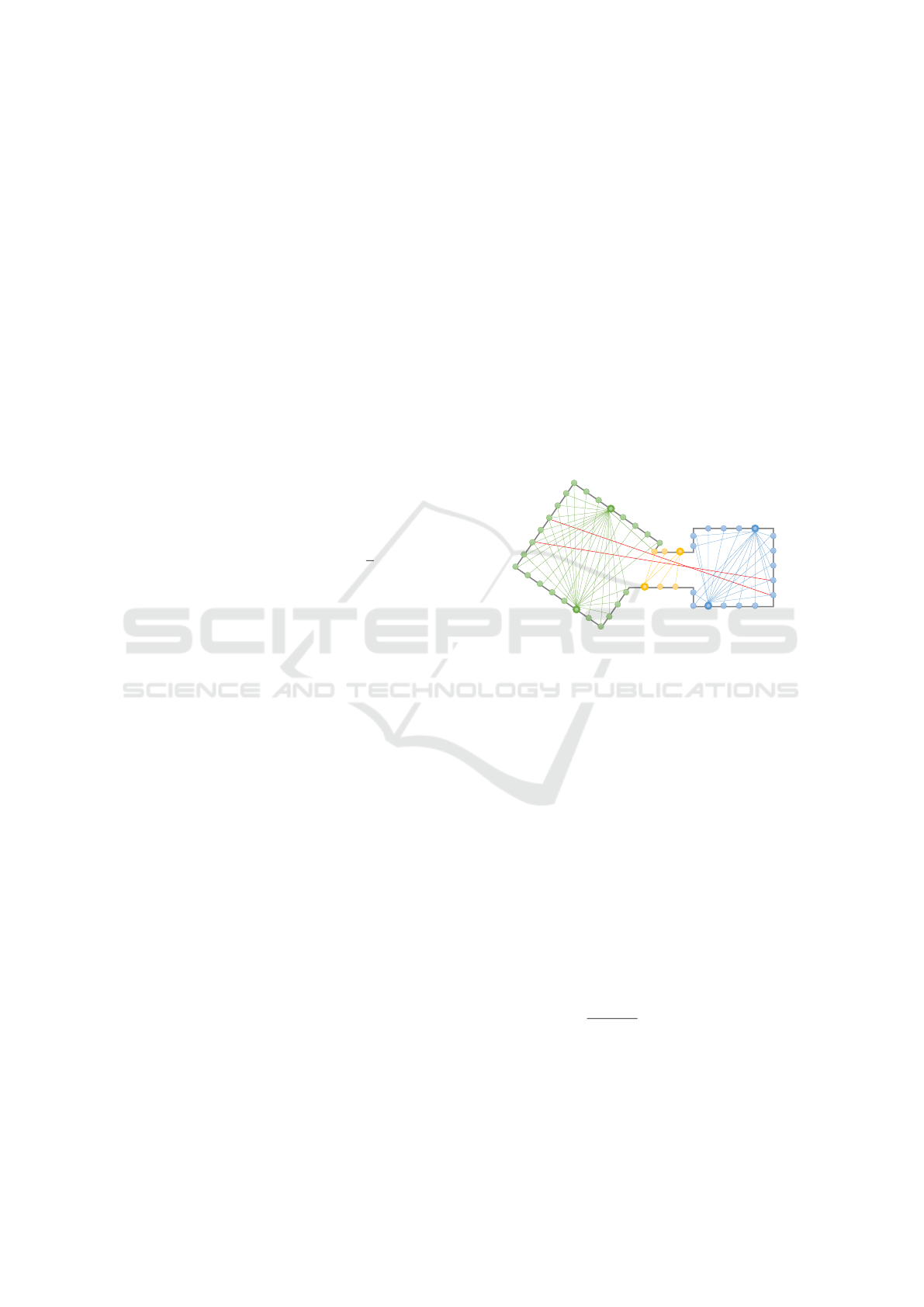
4.3.1 Line-of-Sight (LoS)
The line-of-sight approach for point-cloud clustering
is a variant of the method proposed in (Asafi et al.,
2013). The main idea is to extract a graph G
V
=
(O,LoS(O)) with its vertices being the points of the
input point-cloud O and its edges expressed by the
mapping LoS : O → O ×O with a point set as domain
whose image contains the set of mutually visible point
pairs (see Fig. 2 as an example). This so-called visi-
bility graph has fully or almost fully connected com-
ponents (cliques) where the corresponding model par-
tition is convex or weakly convex. The problem of
finding all maximal cliques in a graph is NP hard, but
we can use Spectral Clustering as an approximation.
Thus, in order to extract these convex model parts, the
graph is clustered, resulting in a set of point-clouds -
one for each convex part. The different steps neces-
Figure 2: A set of sample points O (convex clusters in green,
orange and blue) with exemplary line-of-sights LoS(O) for
each convex cluster (framed circles) of the input model. Red
lines show inter-partition line-of-sights and grey lines cor-
respond to a piece-wise linear approximation of the surface
inferred from the samples. Within a convex cluster, the line-
of-sights form a fully connected graph with the cluster sam-
ples as nodes. Note that when two mutually visible points
belong to the same plane, we do not draw the corresponding
line-of-sight for illustration purpose.
sary for the sketched process of weakly convex clus-
tering are further detailed below.
Proportional Resampling. Since the line-of-sight
computations have quadratic complexity with respect
to the input point-cloud size, the input point-cloud O
s
is re-sampled using Farthest Point Sampling (FPS). In
order to maintain relative point density, as established
by the point structuring step (Section 4.2), for large
surface areas, FPS is applied for points of each plane
separately. The number of remaining points per plane
k
i
is
k
i
= k
|f
sr
(p
i
)|
|O
s
|
, i ∈{1,...,|P|}, (2)
where k is the user-controlled accumulated size of
all per-plane output point-clouds (we used k = 3000
in our experiments) and f
sr
is the mapping between
GRAPP 2021 - 16th International Conference on Computer Graphics Theory and Applications
78
planes in P and points in O
s
. This step results
in a thinned-out point-cloud O
sr
.
Affinity Matrix Computation. Spectral Clustering
is performed on the so-called affinity matrix A which
is the adjacency matrix of the visibility graph G
v
and
reads:
A
i, j
=
(
1, if (v
i
,v
j
) ∈ LoS(O
sr
)
0, otherwise
, (3)
where the line-of-sights LoS(O
sr
) necessary for the
affinity matrix are computed on the structured and
thinned-out input point-cloud O
sr
. A line-of-sight be-
tween two points exists if the segment that connects
these two points does not intersect with the model’s
surface - thus, both points are visible from each other.
Since we don’t have a surface but only a set of points
O
sr
and plane primitives P, it is necessary to approx-
imate the surface in order to perform the necessary
intersection tests. This is done by projecting the set
of points associated to a given plane on that plane
and computing the 2D Alpha Shape (Edelsbrunner
and M
¨
ucke, 1994) of these points. This results in
a piece-wise triangulated surface reconstruction for
each plane. The visibility check for a point-point seg-
ment iterates through all planes and if the segment in-
tersects with a plane, it performs an additional inter-
section test with each triangle associated to that plane.
If an intersection is detected, there is no line-of-sight
between the two points.
In (Asafi et al., 2013) a more efficient technique for
the computation of A is proposed: From each point
o in O
s
, rays (around 50-100) in the opposite direc-
tion of the point’s normal and with a certain random
direction deviation (maximum of 30 degrees) are in-
tersected with the surface approximation. The point
from O
s
which is closest to the first ray-surface in-
tersection is considered to be visible from o. How-
ever, our experiments revealed that this method lead
to affinity matrices which are too sparse and thus to a
low-quality clustering for our data-sets.
Spectral Clustering. Given the affinity matrix A, the
degree matrix D is the diagonal matrix with diagonal
element d
i
=
∑
j
A
i, j
.
The un-normalized Laplacian matrix is given by L =
D −A (this corresponds to the graph Laplacian matrix
when A is the graph adjacency matrix).
There are two commonly used expressions for the
normalized Laplacian matrices:
L
sym
= D
−1/2
LD
1/2
(4)
L
rw
= D
−1
L (5)
L
sym
is the symmetric normalized Laplacian and L
rw
is the so-called random walk normalized Laplacian.
Spectral Clustering is performed by an eigen-analysis
of the normalized Laplacian, followed by a k-Means
clustering of the eigenvectors.
In our experiments, we have found no particular dif-
ferences between using L
sym
or L
rw
in the eigen-
analysis. Additional details and references on Spec-
tral Clustering are provided in (von Luxburg, 2007).
Estimation of the Number of Clusters. Our im-
plementation of Spectral Clustering uses k-Means for
clustering the first k eigenvectors of the graph Lapla-
cian corresponding to A. The number of clusters k is
usually unknown and highly data specific. We tried
several techniques to estimate k (such as a density-
based clustering technique like DBSCAN (Ester et al.,
1996) instead of k-Means, or finding gaps in the se-
quence of eigenvalues of the graph Laplacian), but
none worked consistently in our tests. Instead, we
obtained the best results with an idea introduced in
(Asafi et al., 2013): Spectral Clustering is performed
for different values of k. For each clustering using k
clusters (|C
k
| = k) the clustering quality is measured
by
Q(C
k
) =
1
|O
c
|
2
∑
c∈C
k
|LoS(O
c
)|+α|LoS(O
c
,O
c
)|, (6)
where the image of the mapping LoS : O
1
,O
2
→O
1
×
O
2
contains pairs of points (o
1
,o
2
),o
1
∈ O
1
,o
2
∈ O
2
that are not mutually visible. O
c
is used here as an
abbreviation for the point set O
sr
\ O
c
. The user-
defined weighting parameter α was set to 1 in our ex-
periments. The clustering C
k
with the highest quality
measure Q(C
k
) is selected.
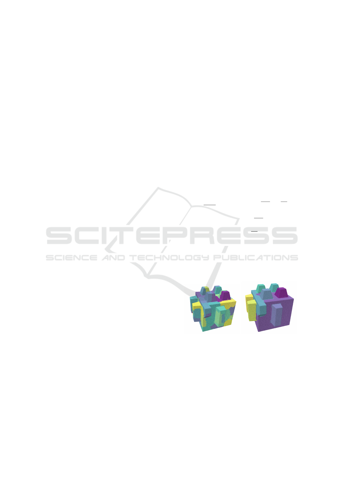
4.3.2 Weakly Convex Segmentation (WCSEG)
Figure 3: Results of intermediate steps of WCSEG. Left:
Over-segmentation. Right: Results after merging.
As an alternative to LoS, we have also experimented
with the Weakly Convex Segmentation (WCSEG) ap-
proach introduced in (Kaick et al., 2014).
Over-segmentation. At first, the input point-cloud is
over-segmented into multiple small patches, obtained
by using a region-growing approach that considers
neighbors, in the k-NN sense, with ”close” normal
vectors (i.e. the angle between the two normal vec-
tors is below some threshold). This step is illustrated
in Fig. 3, left image.
Reconstruction of Convex Polytope Compositions from 3D Point-clouds
79

Neighbor Patch Merging. These multiple small
patches are then merged with a region-growing based
approach, where two neighbor patches are merged if
they are mutually visible (using a notion of visibility
similar to the one described in Section 4.3.1).
Volumetric Merging. The result is a segmentation
of the input point-cloud into weakly convex compo-
nents. The clustering can be further improved by
merging components using a volumetric dissimilarity
score between two components, computed using the
Shape Diameter Function (SDF) value introduced in
(Shapira et al., 2008). An illustration of this step is
provided in Fig. 3, right image.
4.3.3 Structured Point-cloud Assignment
The union of all per-cluster point-clouds may differ
from the set of structured points O
s
depending on
the clustering method used (LoS performs a sub sam-
pling, while we found experimentally that WCSEG
performs better with the full input point cloud). In or-
der to even these differences, points of the structured
point-cloud O
s
are re-distributed among all clusters C
such that
S
c∈C
O
c
= O
s
. This is done using efficient
nearest neighbor queries to find for each point o ∈O
s
the cluster containing the closest point to o among all
points of all clusters.
4.4 Polytope Generation
Based on the weakly convex clustering step, an opti-
mization method is used to find the best combination
of planes to form polytopes for each cluster c ∈ C.
Please note that if the clustering is not perfect (in
the sense that it doesn’t correspond to a convex part),
more than a single polytope can be necessary to fit the
target shape. Thus, our optimization method is capa-
ble to generate a set of convex polytopes per cluster,
rather than a single polytope.
4.4.1 Target Volume Creation
This step and the following ones (Sections 4.4.2 and
4.4.3) are performed for each cluster. Based on the
cluster point-cloud O
c
, a signed distance grid V
c
:
R
3
→R that maps 3D query points to signed distance
values is extracted. V
c
represents the target volume of
the cluster and is generated in order to define a mean-
ingful measure for geometric fitness of a candidate so-
lution (set of polytopes) in the optimization process.
This is done by reconstructing a surface mesh using
Poisson surface reconstruction (Kazhdan et al., 2006)
taking the cluster point-cloud O
c
as input. Then, for
each grid center point, its signed distance to the re-
constructed surface mesh is retrieved and stored. The
signed distance value at an arbitrary query point is ob-
tained by interpolation.
4.4.2 Optimization
In this step, subsets of planes associated with a clus-
ter are combined to form convex polytopes and the
polytope set that best fits the cluster’s target volume
V
c
is selected. This is done by formulating the search
process as a combinatorial optimization problem over
all cluster planes P
c
and solving it via an Evolution-
ary Algorithm. The population is a set of polytope
sets (and each polytope consists of a subset of cluster
planes P
c
).
Objective Function. The objective function to be op-
timized assigns a score to each individual I of the pop-
ulation. It reads
F(I,O
c
,V
c
) = α ·F
g
(I,O
c
) + β ·F
p
(I,V
c
) −γ ·
|I|
n
I max
,
(7)
where F
g
(·,·) is a geometric term, F
p
(·,·) is a per-
polytope geometric term and the last term penalizes
the size of I and is normalized by a user-controlled
maximum value n
I max
. α,β and γ are user-defined
weighting parameters (in our experiments we chose
α = 1, β = 1, γ = 0.1). The geometric term reads
F
g
(I,O
c
) =
1
|O
c
|
∑
o∈O
c
(
1, if min
i∈I
|d
i
(o)| < ε
0, otherwise
,
(8)
where ε is a user-defined minimum value for d
i
(·)
which is the distance of a 3D point to the surface
of polytope i ∈ I. In order to prevent polytope sets
from containing polytopes with large parts being lo-
cated outside of the target volume V
c
, a per-polytope
geometric term is needed. It reads
F
p
(I,V
c
) =
∑
i∈I
1
|H
i
|
∑
h∈H
i
(
1, if V
c
(o
h
) < ε
0, otherwise
, (9)
where H
i
is the set of voxels representing the dis-
cretized volume of polytope i and ε is a user-defined
distance threshold.
Initialization. The initial population is filled
with randomly generated polytope sets containing
polytopes assembled as follows: At first, a plane
is randomly selected from P
c
. Then, a randomly
selected number of neighbor planes are added from
the neighborhood graph G
N
. In some cases, the plane
normals of the the polytope’s faces are not consis-
tently oriented and need to be flipped. For computing
the objective function later on, it is necessary to have
a discretized volume representation (voxel grid) of the
polytope. For that purpose, the polytope’s hull points
GRAPP 2021 - 16th International Conference on Computer Graphics Theory and Applications
80
are computed using the Double Description method
(Fukuda and Prodon, 1996).
Variation Operators. The Crossover operator
exchanges randomly selected sequences of polytopes
in two individuals. The Mutation operator modifies a
single individual and has multiple modes: 1) Alter the
polytope set by randomly replacing polytopes with
newly created random polytopes. 2) Add or remove
random polytopes. 3) Modify existing polytopes by
adding randomly selected planes.
Elite Selection. After each iteration, the polytopes
with the population-wide best per-polytope geometry
scores are selected to form a new individual in
the next iteration. Experiments revealed that this
procedure greatly improves convergence speed.
Termination. The Evolutionary Algorithm termi-
nates if either a certain maximum iteration limit is
reached or if the score of the best solution candidate
has not improved over a certain number of iterations.
4.4.3 Polytope Filtering
The polytopes generated per cluster with a geometry
score lower than a particular threshold are removed
from the result set. In addition, duplicates (polytopes
using the same planes) are eliminated and polytopes
that are fully contained in another polytope are re-
moved as well.
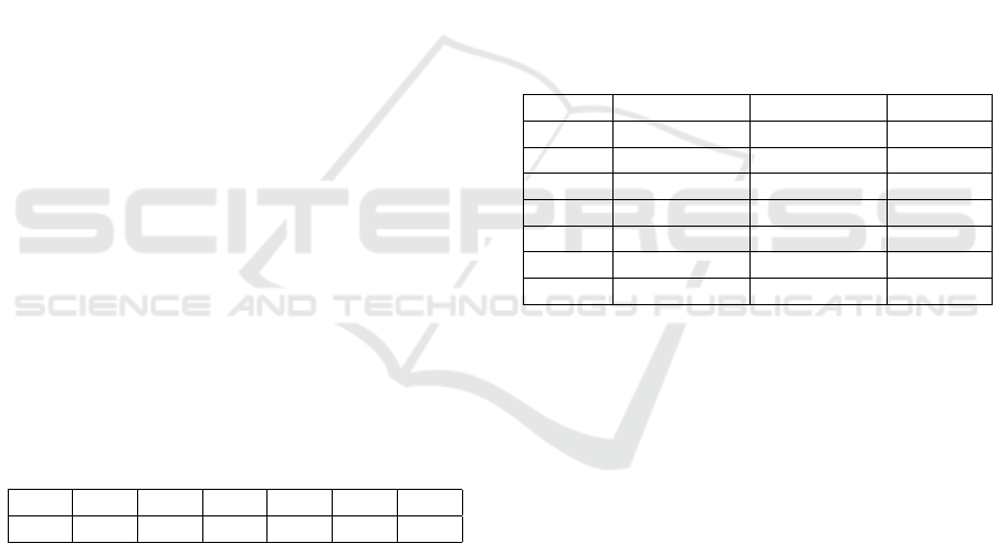
5 EVALUATION
We used seven models in our evaluation - all with dif-
ferent shape and complexity. See Table 1 for the sizes
of the corresponding point-clouds.
Table 1: Point-Cloud sizes for all models.
M1 M2 M3 M4 M5 M6 M7
50k 43k 30k 30k 25k 25k 30k
5.1 Weak Convex Clustering
As described in Section 4.3, we consider two ap-
proaches for weak convex clustering: a variant of LoS
and WCSEG. In the following, we compare their re-
sults on the evaluation data-sets. The results obtained
by these two approaches are summarized in Table 2.
In this table, the term ”Perfect” refers to our quali-
tative opinion of what the correct number of convex
clusters should be for a given model.
As shown in Table 2, the result quality depends on the
input model.
LoS has perfect results for models M3 and M4 where
WCSEG demonstrates a lower quality result (for M4,
see Fig. 4, third column).
On the other hand, WCSEG gives a perfect clustering
result for model M1 whereas LoS is not able to handle
the geometric details (see Fig. 4, first column). The
same is true for model M7 where WCSEG performs
well except for a few incorrectly classified points,
while LoS is not able to find all three clusters (see
Fig. 4, last column).
Model M2 consists of an almost convex main part and
two attached cuboids. Both approaches fail to clas-
sify the smaller details of the main part as indepen-
dent convex clusters (see Fig. 4, second column).
WCSEG is able to find the ’almost’ convex clusters
of M3 whereas LoS fails to find meaningful convex
clusters.
If all polytopes are spatially separated like in model
M6, both LoS and WCSEG find the correct clusters.
Table 2: Number of clusters for both clustering approaches
and all models. The ”-” symbols indicate the amount of
incorrect cluster assignments.
Model LoS WCSEG Perfect
M1 10 (- -) 11 11
M2 3 (- -) 3 11
M3 12 12 (-) 12
M4 12 5 12
M5 1 2 2
M6 2 2 2
M7 2 3 (-) 3
5.2 Pipeline Results
Fig. 6 shows the input point-clouds for our test mod-
els (Fig. 6a) as well as the visual results of the dif-
ferent pipeline steps: Plane Extraction (Section 4.1)
in Fig. 6b, Point-cloud Structuring (Section 4.2) in
Fig. 6c, and Polytope Generation (Section 4.4.2) in
Fig. 6d. For the results of point-cloud structuring
(Fig. 6c), the blue color indicates planar points, the
green color crease points and the brown color corner
points. For each model, the best possible clustering
approach was used (See Sections 4.3 and 5.1). All
models are correctly reconstructed. Only M2 has a
small part of the roof incorrectly recovered (dark red
polytope), but taking into account the low clustering
quality for this model (see Fig. 4, second column), the
resulting polytope collection is actually good. The re-
sult of M6 shows that the pipeline can also correctly
handle disconnected input shapes.
The wall-clock times for the pipeline steps Plane
Extraction, Point-cloud Structuring and Polytope
Generation were measured on a Notebook running a
2.4GHz dual-core CPU with 16GB of RAM and are
Reconstruction of Convex Polytope Compositions from 3D Point-clouds
81
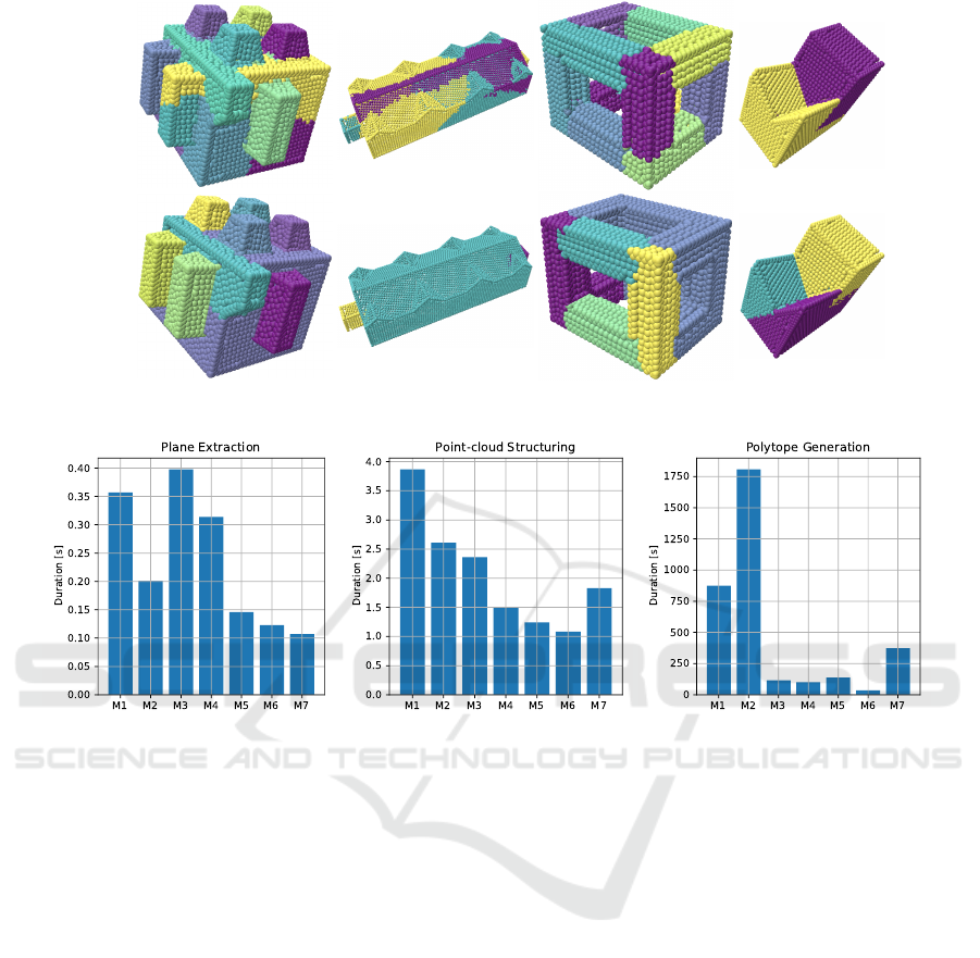
LoSWCSEG
Figure 4: Clustering results for models M1, M2, M4 and M7 (left to right) for LoS (top row) and WCSEG (bottom row).
(a) Plane Extraction. (b) Point-Cloud Structuring. (c) Polytope Generation.
Figure 5: Timings for the main pipeline steps.
shown in Fig. 5a, 5b and 5c. For all models, the
Polytope Generation step takes the most time (see
Fig. 5c), due to the use of an Evolutionary Algo-
rithm (Section 4.4.2). The EA takes the most time
for M2 since it has to generate polytopes for all the
roof details due to the coarse clustering (only 3 clus-
ters found). Interestingly, EA timings for M7 are rel-
atively high. This can be explained as follows: The
Point-cloud Structuring step produces an incomplete
neighborhood graph. Thus, the EA needs to con-
sider all model planes in order to obtain a perfect re-
construction which increases the search space signif-
icantly. By comparison, the timings for the plane ex-
traction step (see Fig. 5a) and the point-cloud structur-
ing step (see Fig. 5b) are negligible. Plane Extraction
takes under 1s for all models, whereas Point-cloud
Structuring takes between 1.1s (M6) and 3.9s (M1).
6 CONCLUSION
This paper introduces a pipeline for the reconstruc-
tion of a solid object as a collection (union) of con-
vex polytopes from a point-cloud. Two different ap-
proaches for partitioning the point-cloud in weak con-
vex clusters are proposed. For each cluster, an EA
is used to find the optimal set of polytopes from the
extracted planes associated to that cluster. As fu-
ture work, we are considering different possible di-
rections: One is to further increase the scalability and
robustness of the convex clustering approaches in or-
der to deal with even larger and more complex point-
clouds. Another direction of future work is to com-
bine this approach with general approaches for CSG
recovery (Fayolle and Pasko, 2016; Friedrich et al.,
2019; Du et al., 2018).
GRAPP 2021 - 16th International Conference on Computer Graphics Theory and Applications
82
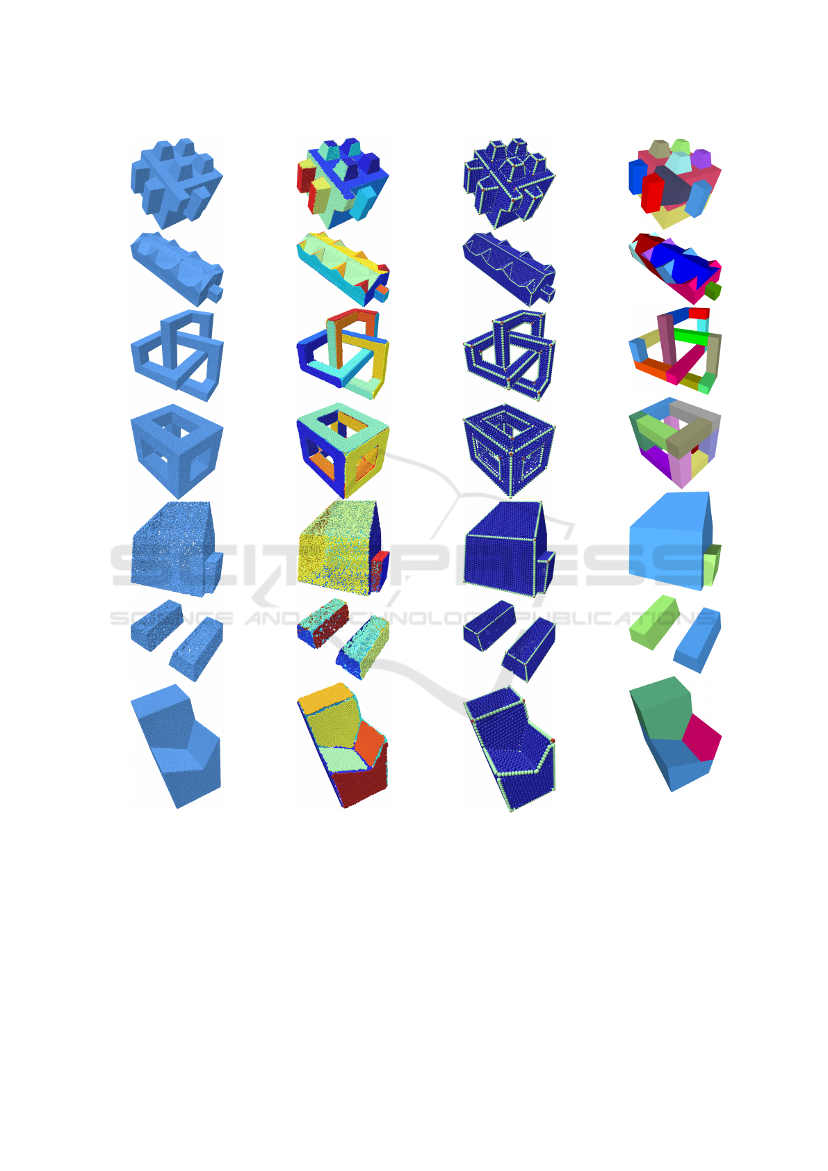
M1M2
M3
M4
M5M6
M7
(a) Input point-cloud.
(b) Points corre-
sponding to fitted
planes.
(c) Structured
point-cloud.
(d) Generated con-
vex polytopes.
Figure 6: Pipeline results for all models.
Reconstruction of Convex Polytope Compositions from 3D Point-clouds
83

ACKNOWLEDGMENTS
We would like to thank the anonymous reviewers for
their valuable comments and suggestions.
REFERENCES
Asafi, S., Goren, A., and Cohen-Or, D. (2013). Weak
convex decomposition by lines-of-sight. Computer
graphics forum, 32(5):23–31.
Benk
´
o, P. and V
´
arady, T. (2004). Segmentation methods
for smooth point regions of conventional engineering
objects. Computer-Aided Design, 36(6):511–523.
Chen, Z., Tagliasacchi, A., and Zhang, H. (2019). Bsp-
net: Generating compact meshes via binary space par-
titioning. arXiv preprint arXiv:1911.06971.
Coumans, E. and Bai, Y. (2016–2019). Pybullet, a python
module for physics simulation for games, robotics and
machine learning. http://pybullet.org.
Deng, B., Genova, K., Yazdani, S., Bouaziz, S., Hinton, G.,
and Tagliasacchi, A. (2019). Cvxnets: Learnable con-
vex decomposition. arXiv preprint arXiv:1909.05736.
Du, T., Inala, J. P., Pu, Y., Spielberg, A., Schulz, A., Rus,
D., Solar-Lezama, A., and Matusik, W. (2018). In-
versecsg: Automatic conversion of 3d models to csg
trees. ACM Trans. Graph., 37(6):1–16.
Edelsbrunner, H. and M
¨
ucke, E. P. (1994). Three-
dimensional alpha shapes. Transactions on Graphics,
13(1):43–72.
Ester, M., Kriegel, H.-P., Sander, J., and Xu, X. (1996).
A density-based algorithm for discovering clusters in
large spatial databases with noise. In Proceedings of
the Second International Conference on Knowledge
Discovery and Data Mining, KDD’96, pages 226–
231. AAAI Press.
Fayolle, P.-A. and Pasko, A. (2016). An evolutionary ap-
proach to the extraction of object construction trees
from 3d point clouds. Computer-Aided Design, 74:1–
17.
Fischler, M. A. and Bolles, R. C. (1981). Random sample
consensus: a paradigm for model fitting with appli-
cations to image analysis and automated cartography.
Communications of the ACM, 24(6):381–395.
Friedrich, M., Fayolle, P.-A., Gabor, T., and Linnhoff-
Popien, C. (2019). Optimizing evolutionary CSG tree
extraction. In Proceedings of the Genetic and Evolu-
tionary Computation Conference, GECCO ’19, page
1183–1191.
Friedrich, M., Illium, S., Fayolle, P.-A., and Linnhoff-
Popien, C. (2020). A hybrid approach for segment-
ing and fitting solid primitives to 3d point clouds.
In Proceedings of the 15th International Confer-
ence on Computer Graphics Theory and Applications
(GRAPP), volume 1, pages 38–48.
Fukuda, K. and Prodon, A. (1996). Double description
method revisited. In Combinatorics and Computer
Science, pages 91–111. Springer Berlin Heidelberg.
Gilbert, E. G., Johnson, D. W., and Keerthi, S. S. (1988).
A fast procedure for computing the distance between
complex objects in three-dimensional space. IEEE
Journal on Robotics and Automation, 4(2):193–203.
Kaick, O. V., Fish, N., Kleiman, Y., Asafi, S., and Cohen-
Or, D. (2014). Shape segmentation by approximate
convexity analysis. ACM Transactions on Graphics
(TOG), 34(1):1–11.
Kaiser, A., Zepeda, J. A. Y., and Boubekeur, T. (2019). A
survey of simple geometric primitives detection meth-
ods for captured 3d data. Computer Graphics Forum,
38(1):167–196.
Kazhdan, M., Bolitho, M., and Hoppe, H. (2006). Poisson
surface reconstruction. In Proceedings of the fourth
Eurographics symposium on Geometry processing,
volume 7 of SGP ’06, page 61–70. Eurographics As-
sociation.
Lafarge, F. and Alliez, P. (2013). Surface reconstruction
through point set structuring. Computer Graphics Fo-
rum, 32(2pt2):225–234.
Li, M., Wonka, P., and Nan, L. (2016). Manhattan-world ur-
ban reconstruction from point clouds. In ECCV, pages
54–69.
Li, Y., Wu, X., Chrysathou, Y., Sharf, A., Cohen-Or, D.,
and Mitra, N. J. (2011). Globfit: Consistently fitting
primitives by discovering global relations. ACM trans-
actions on graphics (TOG), 30(4):1–12.
Monszpart, A., Mellado, N., Brostow, G. J., and Mitra, N. J.
(2015). RAPter: Rebuilding man-made scenes with
regular arrangements of planes. ACM Trans. Graph.,
34(4):1–12.
Musialski, P., Wonka, P., Aliaga, D. G., Wimmer, M., Gool,
L., and Purgathofer, W. (2013). A survey of urban re-
construction. Comput. Graph. Forum, 32(6):146–177.
Nan, L. and Wonka, P. (2017). Polyfit: Polygonal surface
reconstruction from point clouds. In 2017 IEEE In-
ternational Conference on Computer Vision (ICCV),
pages 2372–2380.
Oesau, S., Lafarge, F., and Alliez, P. (2016). Planar Shape
Detection and Regularization in Tandem. Computer
Graphics Forum, 35(1):203–215.
Schnabel, R., Wahl, R., and Klein, R. (2007). Efficient
ransac for point-cloud shape detection. Computer
graphics forum, 26(2):214–226.
Shapira, L., Shamir, A., and Cohen-Or, D. (2008). Con-
sistent mesh partitioning and skeletonisation using
the shape diameter function. The Visual Computer,
24(4):249–259.
Tulsiani, S., Su, H., Guibas, L. J., Efros, A. A., and Malik,
J. (2017). Learning shape abstractions by assembling
volumetric primitives. In Proceedings of the IEEE
Conference on Computer Vision and Pattern Recog-
nition, pages 2635–2643.
V
´
arady, T., Benko, P., and Kos, G. (1998). Reverse en-
gineering regular objects: simple segmentation and
surface fitting procedures. Int. J. of Shape Modeling,
3(4):127–141.
von Luxburg, U. (2007). A tutorial on spectral clustering.
Statistics and Computing, 17:395–416.
Xiao, J. and Furukawa, Y. (2014). Reconstructing the
world’s museums. International Journal of Computer
Vision, 110(3):243–258.
GRAPP 2021 - 16th International Conference on Computer Graphics Theory and Applications
84
