Acoustic Leak Detection in Water Networks

Robert M

uller

1 a

, Steffen Illium

1 b

, Fabian Ritz

1 c

, Tobias Schr

oder

, Christian Platschek

org Ochs

and Claudia Linnhoff-Popien

1 d

Mobile and Distributed Systems Group, LMU Munich, Germany

Stadtwerke M

unchen GmbH, Germany

Keywords:

Leak Detection, Water Networks, Acoustic Anomaly Detection, Applied Machine Learning.

Abstract:

In this work, we present a general procedure for acoustic leak detection in water networks that satisﬁes multiple

real-world constraints such as energy efﬁciency and ease of deployment. Based on recordings from seven

contact microphones attached to the water supply network of a municipal suburb, we trained several shallow

and deep anomaly detection models. Inspired by how human experts detect leaks using electronic sounding-

sticks, we use these models to repeatedly listen for leaks over a predeﬁned decision horizon. This way we

avoid constant monitoring of the system. While we found the detection of leaks in close proximity to be a

trivial task for almost all models, neural network based approaches achieve better results at the detection of

distant leaks.

1 INTRODUCTION

Leakage is one of the main causes for water loss in

water supply and distribution networks. Undetected

leaks, which usually occur due to corrosion and soil

movement, may have extensive negative effects on the

surrounding infrastructure, customer convenience and

ﬁnancial proﬁt. Contributing to this problem is the

fact that it can take a considerable amount of time un-

til a leak is detected, localized and countermeasures

are put into place.

In the UK, approximately 3200 Million liters of

water are wasted due to leakages in water networks

every day (WaterUK, ), a disproportionately high

value with regard to climate change and a shortage

of drinking water in many countries. Greater efforts

are needed to minimize water loss through leakages.

A reliable indicator for substantial water loss is

the deviation of the zero-consumption status in a bal-

ance area at night. But if a leakage is more subtle, it

is usually not detected until water emerges from the

surfaces and residents report the issue.

Locating the source by means of the acoustic emis-

sion from exiting water is one the predominantly used

https://orcid.org/0000-0003-3108-713X

https://orcid.org/0000-0003-0021-436X

https://orcid.org/0000-0001-7707-1358

https://orcid.org/0000-0001-6284-9286

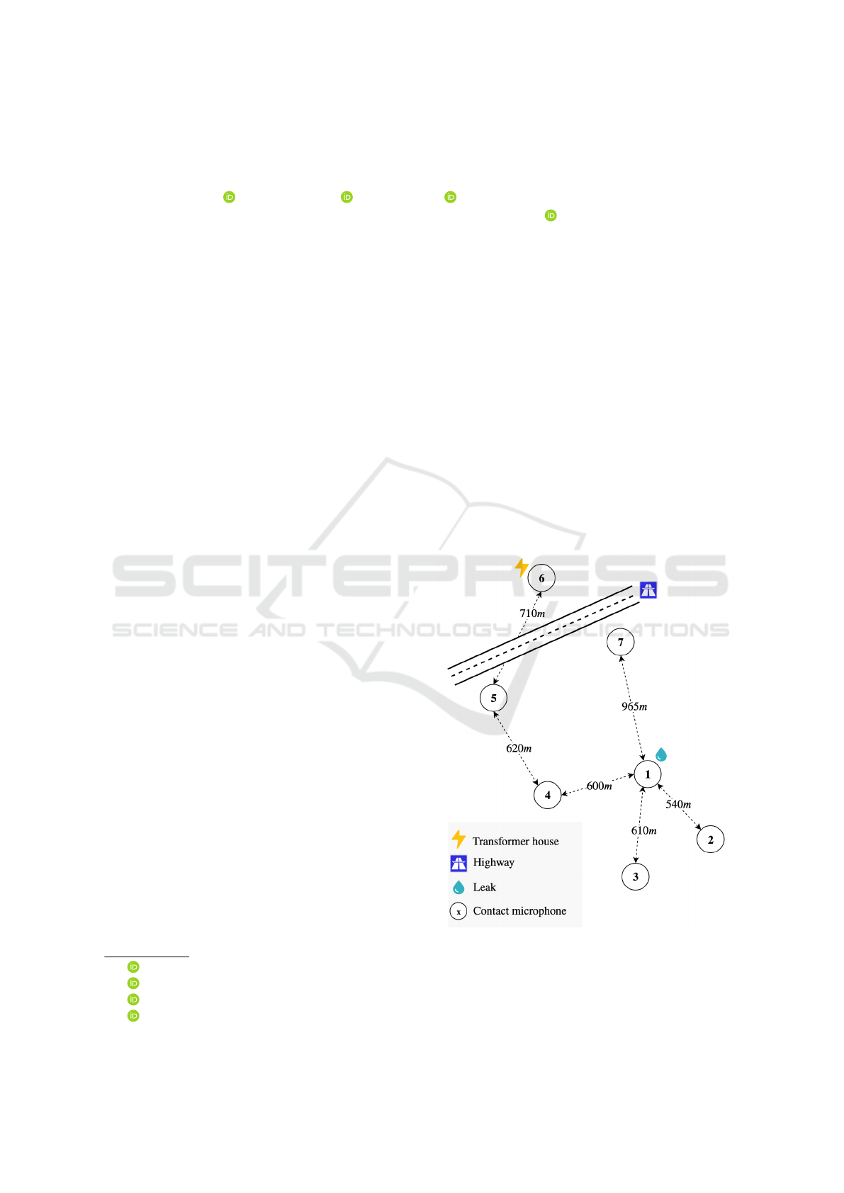
Figure 1: Simpliﬁed map of the location of each contact

microphone and signiﬁcant objects in their neighborhood.

For each contact microphone, we depict the distance of the

shortest pipeline link to another contact microphone. Note

that distance is give n in meters of water pipe.

306

Müller, R., Illium, S., Ritz, F., Schröder, T., Platschek, C., Ochs, J. and Linnhoff-Popien, C.

Acoustic Leak Detection in Water Networks.

DOI: 10.5220/0010295403060313

In Proceedings of the 13th International Conference on Agents and Artiﬁcial Intelligence (ICAART 2021) - Volume 2, pages 306-313

ISBN: 978-989-758-484-8

approaches (El-Zahab and Zayed, 2019). The process

is as follows:

1) Leak Noise Correlation: Liquid escaping a pipe

creates shock waves that cause the pipe to vibrate, re-

sulting in a characteristic leak sound. At least two

sensors are attached to the pipe around the presumed

leak location. By analyzing the variation in propaga-

tion times of the leak’s acoustic emission between the

sensors, the location is further narrowed down. This

approach requires infrastructural knowledge, such as

pipe material, diameter, length and corresponding

sound velocities.

2) Electro-acoustic Method: To further pinpoint the

location, human leak detection experts search for leak

noises using electronic sounding sticks. A leak can

be localized by exploiting the fact that leak sounds

become more dominant as the expert approaches the

leak. The process relies on trained human experts

and requires a solid estimate of the leakage location

as ﬁnding the ﬁrst evidence might otherwise become

very time consuming.

In this work, we aim to automatize the electro-

acoustic method utilizing machine learning. We

record normal operation data using seven contact mi-

crophones attached on various parts of the water sup-

ply network in a suburban area of Munich. Subse-

quently, we train several unsupervised anomaly de-

tection models and embed these into a broader proce-

dure that satisﬁes several real world constraints, such

as energy consumption and limited bandwidth. Our

approach can be understood as a ﬁrst step towards a

fully automatized leak detection system that does not

need to wait for leak aftereffects to appear. More-

over, our approach is data-driven and does not require

a detailed mathematical model of the water network’s

inner workings.

The rest of the paper is structured as follows: In

Section 2 we brieﬂy review related work. Then we

motivate and propose a general procedure for acoustic

leak detection in Section 5. In Section 4 we describe

the data acquisition process followed by the descrip-

tion of the experimental setup and its evaluation. We

close by summarizing our ﬁndings in Section 6 and

laying out future work in Section 7

2 RELATED WORK

Related approaches of acoustic leak detection are

mostly based on cross-correlation (Muggleton and

Brennan, 2004; Gao et al., 2017), wavelet trans-

forms (Ni and Iwamoto, 2002; Ting et al., 2019),

Support-Vector-Machines (Kang et al., 2017; Cody

et al., 2017) or neural networks (Kang et al., 2017;

Chuang et al., 2019; Cody et al., 2020). Other meth-

ods combine acoustic data with additional sensory

measurements (Stoianov et al., 2007). Their perfor-

mance depends on the pipe network material (e.g.

polyethylene or metal). However, none of these ap-

proaches directly matches the setup and constraints of

this work as experiments are mostly carried out under

laboratory conditions and only study a single algorith-

mic approach. Other physical phenomena that occur

in presence of a leak can also be taken advantage of,

e.g. using thermography, ground penetration radar or

pressure-based methods. An exhaustive summary can

be found in (Adedeji et al., 2017; Chan et al., 2018).

Apart from leak detection, the broader ﬁeld of

acoustic anomaly detection has recently gained trac-

tion.

Most of the recent work in the ﬁeld is based upon

Deep-Autoencoders (AEs). An AE learns to recon-

struct its input from a compressed latent representa-

tion. Unseen, anomalous data is assumed to have a

higher reconstruction error. The approaches mostly

differ in the architecture used.

Duman et al. (Duman et al., 2019) use a deep con-

volutional AE on the spectrograms of sounds from in-

dustrial processes. In (Meire and Karsmakers, 2019)

the authors also conclude that convolutional AEs per-

form well on the task of acoustic anomaly detection

while they have also found the One-Class Support

Vector Machine to be a strong competitor. In the same

vein, M

uller et al. (M

uller et al., 2020) use pretrained

convolutional neural networks for feature extraction

and train various traditional anomaly detection mod-

els. Other work (Marchi et al., 2015; Li et al., 2018;

Nguyen et al., 2019) explicitly takes the sequential

nature of sound into account by training a recurrent

AE based on Long-Short-Term Memory. Koizumi et

al (Koizumi et al., 2017) use a more traditional Feed-

Forward AE in conjunction with a novel loss function

based on statistical hypothesis testing. This approach

requires the simulation of anomalous sounds by us-

ing rejection sampling. Recently, Suefusa et al. (Sue-

fusa et al., 2020) proposed to alter the input an AE

receives to improve the detection of non-stationary

sounds. Instead of predicting all spectrogram frames,

they remove the center frame and use it as prediction

target thereby alleviating the difﬁculty of predicting

the edge frames.

Another line of work investigates upon methods

that operate directly on the raw waveform (Hayashi

et al., 2018; Rushe and Namee, 2019). WaveNet-

like (Oord et al., 2016) generative architectures that

utilize causal-dialated convolutions are used to pre-

dict the next sample. The prediction error serves as

the anomaly score.

Acoustic Leak Detection in Water Networks

307

3 MOTIVATION AND PROBLEM

DEFINITION

An automated leak detection system should be

energy efﬁcient, easy to deploy and easy to update.

We derive the problem deﬁnition from the following

deployment scenario: Small battery driven IoT

devices record sounds from contact microphones

upon request from a central control unit. During a

predeﬁned period, sounds are periodically recorded

for a short time frame (2-5s). Afterwards, the col-

lection of short audio sequences is transmitted to the

central control unit via a low energy, low bandwidth

radio network (SWM, 2018). This reduces the high

energy and bandwidth consumption that constant

monitoring would cause. The central control unit

can then put all received measurements in context to

decide whether a leak is present or not. Moreover,

using a central control unit makes updating the

system (e.g. changing the algorithm or retraining the

model) more feasible. This approach is inspired by

how human leak detection experts make decisions

using electronic sounding sticks. After attaching

the stick on to a hydrant connection, the expert

listens carefully for up to ten seconds. When facing

audible noise emitted by infrastructure, agriculture

or industry, the process is repeated until an accurate

decision can be made. For precise leak localization,

various hydrant or valve connections in the area are

checked accordingly. Increasing leak sounds indicate

a decreased distance to the leak. In this work, we

focus on leak detection and leave localization for

future work. Our approach is formulated as follows:

Problem Deﬁnition 1. Let X be some representation

of an h minute recording from a contact microphone

on a water pipe. Further, let F

: Y −→ R

be some

trainable function with parameters θ where Y is a

sample of X with a length of t seconds. Apply F

m different sections of X to obtain a vector ∈ R

positive real valued anomaly scores. To compute a

single anomaly score for X, combine the measure-

ments using an aggregation function φ : R

−→ R

Find (F

, φ, h, t, m) such that the anomaly scores for

leak sections are higher than the anomaly-scores for

no-leak sections.

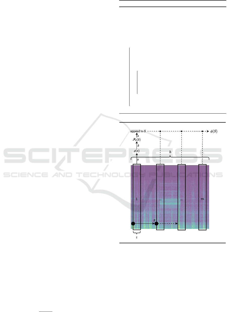
The accompanying algorithm is depicted in Algo-

rithm 1. Note that the sampling timepoints are equally

distributed across the whole recording (Line 3), i.e.

linspace returns the set

{bi ∗

(h − t)

c|i ∈ 1, . . . m}

Algorithm 1: Acoustic Leak Detection.

Input: Audio recording X

Parameters: Score func. F

, Aggregation

func. φ, Number of samples m,

Sample length t, preprocessing

func. ρ

Output: Anomaly Score for X

1 begin

2 h ←− length(X)

3 P ←− linspace(0, h − t, m)

4 S ←− [ ]

5 for p in P do

6 x ←− X [p : p +t]

7 ˜x ←− ρ(x)

8 s ←− F

( ˜x)

9 append s to S

10 end

11 return φ(S)

12 end

Figure 2: Visualization of the most important aspects of our

acoustic leak detection approach.

and each sample is preprocessed (Line 7) to ﬁt the do-

main of the score function (e.g. spectrum, raw-audio

or feature vector). We also depict the most important

aspects of the method visually in Figure 2 To obtain

enough leak sound recordings for supervised learning,

one would have to artiﬁcially create a vast amount of

leaks. Furthermore, for these recordings to contain

enough diversity, this would have to be done on vari-

ous sections of the water network. Due to the ﬁnancial

ICAART 2021 - 13th International Conference on Agents and Artiﬁcial Intelligence

308

and environmental issues that would arise, we assume

that F

is trained on normal operation data only.

4 DATA ACQUISITION

For data acquisition, a suburban part of Munich with

little trafﬁc was chosen as a testing ground. Seven

contact microphones were directly attached onto hy-

drants of an iron pipe network (∅ 100mm). Figure 1

shows a simpliﬁed map marking the locations of the

microphones as well as signiﬁcant objects in the sur-

rounding area that might inﬂuence the quality of the

recordings. Sounds were recorded for three months.

To avoid excessively high signals (overdrive), we

kept the pre-ampliﬁer, equalizer and post-ampliﬁer

neutral, effectively recording sounds ”as-is” and dis-

abling the dynamic sensitivity adjustment. This leads

to the recordings having a headroom of 24 dB on av-

erage. All contact microphones are designed to record

sounds reliably between 300Hz and 3000Hz. During

the time of recording, a medium sized water leakage

occurred in close proximity (≈ 20m) to contact mi-

crophone one (see Figure 1). The leak was present

for 28 days and was ﬁxed thereafter. Furthermore, we

conducted various ﬁeld tests. We simulated a leakage

by opening a hydrant near contact microphone ﬁve

and attached a contact microphone to hydrant connec-

tions between contact microphone four and ﬁve every

100 meters. Overall, we were neither able to hear the

leak nor able to observe typical leak patterns in the

frequency spectrograms beyond a distance of 600 me-

ters.

5 EVALUATION

In this section, we conduct various experiments to

ﬁnd an appropriate setting of (F

, φ, h, t, m). First we

introduce the dataset followed by a brief discussion of

the anomaly detection models that were used. Finally,

we present the experiments and results.

5.1 Methodology and Dataset

The evaluation set up is designed to line up with

Problem Deﬁnition 1. We use 600 hours of normal

operation recordings equally sampled from all contact

microphones. Sounds were recorded in mono with

a sampling rate of 16 kHz and a bit depth of 16 bit.

A band-pass ﬁlter is applied to remove information

above and below the contact microphone’s supported

frequencies. For training, we split the data into

t = {2s, 5s} long audio samples with no overlap.

These values are at the lower end of how long a

human expert listens using a sounding stick. Samples

are then preprocessed (Algorithm 1, Line 7) by either

computing its mel-spectrogram or extracting eight

spectral features (chromagram, spectral centroid,

spectral bandwidth, spectral contrast, spectral roll

off, spectral ﬂatness, zero-crossing rate and the

root-mean-square value) which we have identiﬁed

to be good descriptors of a leak during early stages

of research. Each feature-vector is standardized by

subtracting the mean and dividing by the standard-

deviation of the individual features. Figure 3 provides

more insights into the characteristics of the dataset.

To evaluate the ability of our approach to differentiate

between leak and no-leak, we use the following two

datasets:

Leak in Close Proximity: To measure the

ability to detect leaks in close proximity to a contact

microphone, we select ﬁve consecutive days during

which a leak was present in close proximity to contact

microphone 1. For each day, we use the recordings

from contact microphone 1 and one other contact

microphone. This results in a balanced evaluation

dataset with an equal number of leak and no-leak

recordings.

Leak in the Distance (Synthetic): This setting

measures how well a leak can be detected when it is

farther away from a contact microphone. As we were

only able to obtain recordings from a leakage near a

single contact microphone, we mixed normal record-

ings with leak sounds having a high Signal-to-Noise

Ratio of +24dB. Note that here noise stands for the

leak sounds. Doing so yields synthetically generated

recordings that resemble the characteristics of a leak-

age in the distance (Section 4). Synthetically creating

anomalous recordings is a common approach when

anomalous data is scarce (Duman et al., 2019; Puro-

hit et al., 2019; Koizumi et al., 2019; Socor

o et al.,

2015; Stowell et al., 2015; Nakajima et al., 2016).

We select 96 hours of no-leak recordings from contact

microphones two and three. 48 hours of these record-

ings were mixed with randomly sampled leak sounds

taken from a time-span between 0a.m. - 4a.m. This

time-span was chosen as it yields pure leak sounds

with very little noise.

5.2 Anomaly Detection Models

To compute anomaly scores for each individual

sample (Algorithm 1, Line 8) we use various density

estimation, ensemble models and deep neural net-

works. Models can be further subdivided according

Acoustic Leak Detection in Water Networks

309

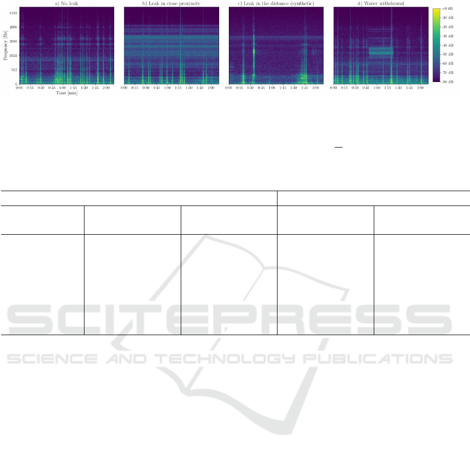
Figure 3: Four Mel-spectrograms depicting a) normal operation, b) a leak in close proximity, c) a synthetically generated

distant leak and d) water withdrawal. Spikes are caused by cars driving over the hydrant cover above the contact microphones.

However, other recordings may also contain footsteps, animal noises or interfering noises due to a nearby transformer house.

A leak is characterized by high energy in the upper frequencies. This pattern becomes less dominant as the distance to the

leak increases and vanishes after ≈ 600m. The leak shown in b) has a throughput of ≈ 300

Table 1: Average AUCs with standard deviations (over 5 seeds) for different settings of F , h and t where φ = median, m =

20, h = 30min and m = 40, h = 60min.

Leak in close proximity Leak in the distance (synthetic)

Decision horizon h 30min 60min 30min 60min

Sample length t 2s 5s 2s 5s 2s 5s 2s 5s

GMM 74.8±2.5 88.0±1.3 74.6±2.1 87.6±1.6 64.0±5.5 68.7±0.0 68.4±1.0 70.0±1.2

B-GMM 78.7±3.7 88.1±2.4 78.8±4.0 87.7±2.6 64.0±5.1 70.5±1.8 69.3±1.2 72.5±2.9

IF 98.6±0.0 98.8±0.0 98.8±0.0 100±0.0 41.4±0.0 42.5±1.8 41.0±1.5 42.3±2.3

RealNVP 98.6±2.0 98.0±3.6 99.0±1.3 98.1±3.7 75.2±2.7 76.1±2.5 77.1±2.8 78.3±3.1

DCAE 98.2±0.0 98.9±0.0 99.8±0.0 100±0.0 75.1±1.5 73.4±5.0 76.1±2.1 76.0±3.3

AAE 98.9±0.0 99.0±0.0 99.8±0.0 99.8±0.0 75.0±4.4 69.9±3.2 77.0±5.2 71.6±2.4

AVB 98.1±0.5 99.5±0.1 99.6±0.5 100±0.0 76.9±3.4 75.5±2.7 78.9±3.7 77.5±2.8

to the input they receive.

Mel-spectrogram Input: A mel-spectrogram is

a logarithmically scaled spectrogram to better align

with how humans perceive sound. We compute the

mel-sepctograms with 64 mels, fft window = 2048

frames, hop length = 512 frames and normalize them

to lie in the range [0, 1]. We also experimented with

other settings but have found all methods to be robust

against these parameters. The following deep neural

networks are trained: i) Deep Convolutional Auto

Encoder (DCAE) A neural network that compresses

the input into a low dimensional representation and

then reconstructs the input from this representation.

We use [4, 16, 32] convolution ﬁlters with 2 × 2 max-

pooling in-between each layer with ReLU (Agarap,

2018) as activation function. We train for 100 epochs

with a batch size of 128, a L2 weight penalty of

−6

and optimize the AE using ADAM (Kingma

and Ba, 2014) with a learning rate of 0.0001. For

reconstruction, the inverse operations (deconvolution

and up sampling) are applied in reverse order. ii)

Adversarial Auto Encoder (AAE) (Makhzani et al.,

2015) Adversarially trained DCAE such that the

latent space spanned by the bottleneck features

matches the prior distribution N (0, I). iii) Adver-

sarial Variational Bayes (Mescheder et al., 2017)

Adversarially trained variational DCAE.

Feature-Vector Input: Here we extract eight

spectral features (see Section 5) for each sample. The

resulting feature vectors are used to train i) Gaus-

sian Mixture Model (GMM) A density estimation al-

gorithm that models the underlying probability distri-

bution as a mixture of Gaussians. Parameters are es-

timated using expectation-maximization. We use 16

mixture components with diagonal covariance matri-

ces. ii) Bayesian Gaussian Mixture Model (B-GMM)

In contrast to a GMM, this model is trained using

variational inference. We use the same parameters

as for the GMM. iii) RealNVP (Dinh et al., 2017) A

sequence of invertible transformations modeled by a

neural network that can directly compute the proba-

bility density of the data. The approach is based on

normalizing ﬂows. We use 3 coupling layers, a hid-

den dimension of 150, a batch size of 768 and assume

a normal distribution with zero mean and unit vari-

ance as base distribution. All of the methods above

use the log-probability of a sample as normality score.

iv) Isolation Forest (IF) (Liu et al., 2008) Recursively

ICAART 2021 - 13th International Conference on Agents and Artiﬁcial Intelligence

310

partitions the feature space. The number of splits

needed to isolate a data point is used as normality

score. We use 120 base estimators.

Model performance is measured with the Area

Under the Receiver Operating Characteristics (AUC)

which quantiﬁes how well a model can distinguish be-

tween leak and no-leak across all classiﬁcation thresh-

olds. The AUC is the standard metric to evaluate

anomaly detection models across many domains (Ag-

garwal, 2015; Chalapathy and Chawla, 2019) as it

yields a complete sensitivity/speciﬁcity report. The

evaluation setup follows (Ruff et al., 2018).

5.3 Choosing the Model

The most important aspect of our approach is to

choose a suitable score function F

. The datasets

presented in Section 5 are split into consecutive h =

30min and h = 60min long recordings. On each of

these recordings, we run Algorithm 1 independently

to obtain a single anomaly score. Here we chose the

median as aggregation function φ due to its robustness

against outliers

and evaluate across all models from

Section 5.2 with t = 2 and t = 5. We set m = 20 and

m = 40 for h = 30 min and h = 60 min, respectively.

Model parameters were determined using a small de-

velopment set.

Results are depicted in Table 1. In the case of

Leak in close proximity the performance of GMM and

B-GMM is signiﬁcantly worse compared to all other

models. Interestingly, AUC-scores for GMM and B-

GMM increase by approximately 12% when t = 5.

This ﬁnding carries over the second setting as well.

When h = 60 and t = 5 IF, DCAE and AVB reach

perfect scores. Generally, the setting can be consid-

ered trivial for IF, RealNVP, DCAE, AVB and AAE.

Note that in case of the AAE and AVB we also tried

using the log-probability of the latent representation

but the reconstruction error turned out to yield better

results.

Results for Leak in the distance (synthetic) paint

a different picture. In this setting, the differences be-

tween inlier and outlier are more subtle and therefore

considerably harder to detect. IF fails completely on

this task due to the reduced distance between inlier

and outlier in feature space. The number of splits is

the same for almost all samples and mostly depends

on the random splitting points. Moreover, we observe

general superiority of the neural network (NN) based

methods RealNVP, DCAE, AVB and AAE indicating

The median showed the best results compared to other

aggregation functions like the mean. Using only the most

normal sample (min-pooling) leads to a comparable, but

worse performance.

that NNs better reveal the more subtle differences. On

2s, Mel-spectrogram based AVB performs best and on

5s RealNVP outperforms all other methods. We ob-

served that auto encoders work best with a small bot-

tleneck as this limits their ability to generalize over

leak patterns based on water withdrawal. Moreover,

we can verify that the extracted feature set is indeed

a good leak indicator as ist shows strong performance

when used in conjunction with NN based RealNVP.

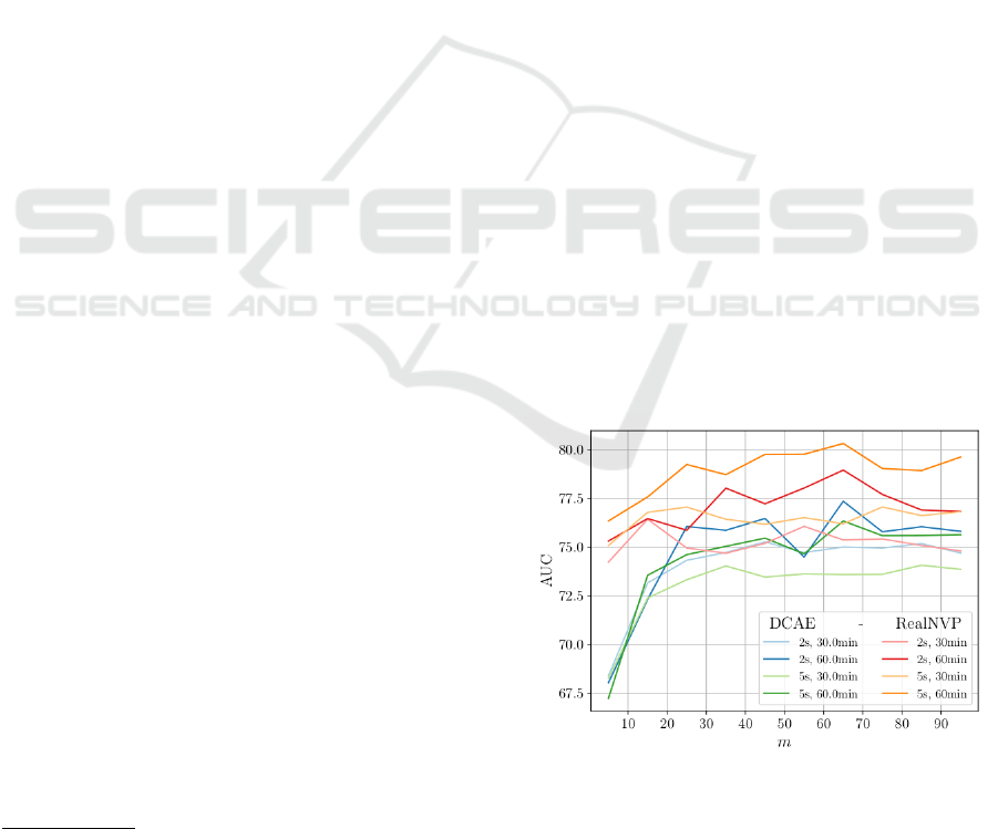
5.4 Choosing the Number of Samples

In this experiment, we evaluate upon the inﬂuence

of the number of samples on the model perfor-

mance. In ﬁgure 4, we vary the number of sam-

ples m from 5 to 105 in steps of 10 samples. We

evaluate across all combinations of decision horizon

h ∈ {30min, 60min} and sample length t ∈ {2s, 5s}

on Leak in the distance (synthetic) with φ=median.

For better clarity, we only show results for RealNVP

and DCAE.

In Figure 4, we observe that using less than 15

samples yields signiﬁcantly worse performance. Re-

sults stabilize thereafter and peak performance is

achieved at m = 65 for most settings. We conclude

that increasing the number of samples has a positive

effect on the performance because it makes the de-

cision less dependent on individual samples. More

samples better represent the underlying distribution as

a leak is characterized by a constantly present acous-

tic pattern. In contrast to a streaming approach, only

a fraction of all possible measurements has to be con-

sidered as we did not observe a substantial increase in

performance by considering even more samples.

Figure 4: Performance comparison for m =

{5, 15, 25, . . . 105} on Leak in the distance (synthetic).

Each value is the average AUC over 5 seeds.

Acoustic Leak Detection in Water Networks

311

6 CONCLUSION

In this work, we presented a general procedure for

leak detection in water networks that satisﬁes real-

world constraints and provided a thorough evaluation

of different parameter settings. While a leak in close

proximity to a contact microphone is trivial for most

scoring functions, neural network based approaches

yielded superior results with respect to the detection

of a (synthetic) leak in the distance. Additionally, we

found that it is not necessary to constantly monitor

the system. It sufﬁces to consider a fraction of the

recordings during a predeﬁned decision horizon.

7 FUTURE WORK

Future work might investigate further upon differ-

ent scoring functions, e.g. by taking the sequen-

tial nature of the recordings into account. Other av-

enues worth exploring are more sophisticated sam-

pling and aggregation strategies. The extension of

our approach to leak localization (e.g. via trilater-

ation) represents the next logical step. Moreover,

instead of training a single model on data from all

contact-microphones, one might train separate mod-

els. Another possibility would be to use weight shar-

ing and condition (Huang and Belongie, 2017) the

model on the contact-microphone ID or on features

of their surrounding. Another important aspect that

still remains to be investigated, is how to update the

model when new data (possibly collected in another

area) arrives (Koizumi et al., 2020).

ACKNOWLEDGMENTS

This work is part of the research project ErLoWa

which was carried out in cooperation with Stadtwerke

unchen GmbH.

REFERENCES

Adedeji, K. B., Hamam, Y., Abe, B. T., and Abu-Mahfouz,

A. M. (2017). Towards achieving a reliable leakage

detection and localization algorithm for application in

water piping networks: An overview. IEEE Access,

5:20272–20285.

Agarap, A. F. (2018). Deep learning using rectiﬁed linear

units (relu). arXiv preprint arXiv:1803.08375.

Aggarwal, C. C. (2015). Outlier analysis. In Data mining,

pages 237–263. Springer.

Chalapathy, R. and Chawla, S. (2019). Deep learning

for anomaly detection: A survey. arXiv preprint

arXiv:1901.03407.

Chan, T., Chin, C. S., and Zhong, X. (2018). Review of cur-

rent technologies and proposed intelligent methodolo-

gies for water distributed network leakage detection.

IEEE Access, 6:78846–78867.

Chuang, W.-Y., Tsai, Y.-L., and Wang, L.-H. (2019). Leak

detection in water distribution pipes based on cnn with

mel frequency cepstral coefﬁcients. In Proceedings of

the 2019 3rd International Conference on Innovation

in Artiﬁcial Intelligence, pages 83–86.

Cody, R., Narasimhan, S., and Tolson, B. (2017). One

Class SVM – Leak Detection in Water Distribution

Systems’.

Cody, R. A., Tolson, B. A., and Orchard, J. (2020). De-

tecting leaks in water distribution pipes using a deep

autoencoder and hydroacoustic spectrograms. Journal

of Computing in Civil Engineering, 34(2).

Dinh, L., Sohl-Dickstein, J., and Bengio, S. (2017). Den-

sity estimation using real NVP. In 5th International

Conference on Learning Representations, ICLR 2017.

Duman, T. B., Bayram, B., and

Ince, G. (2019). Acoustic

anomaly detection using convolutional autoencoders

in industrial processes. In International Workshop on

Soft Computing Models in Industrial and Environmen-

tal Applications, pages 432–442. Springer.

El-Zahab, S. and Zayed, T. (2019). Leak detection in wa-

ter distribution networks: an introductory overview.

Smart Water, 4(1):5.

Gao, Y., Brennan, M. J., Liu, Y., Almeida, F. C., and

Joseph, P. F. (2017). Improving the shape of the cross-

correlation function for leak detection in a plastic wa-

ter distribution pipe using acoustic signals. Applied

Acoustics, 127:24–33.

Hayashi, T., Komatsu, T., Kondo, R., Toda, T., and Takeda,

K. (2018). Anomalous sound event detection based on

wavenet. In 2018 26th European Signal Processing

Conference (EUSIPCO), pages 2494–2498. IEEE.

Huang, X. and Belongie, S. (2017). Arbitrary style transfer

in real-time with adaptive instance normalization. In

Proceedings of the IEEE International Conference on

Computer Vision, pages 1501–1510.

Kang, J., Park, Y.-J., Lee, J., Wang, S.-H., and Eom, D.-

S. (2017). Novel leakage detection by ensemble cnn-

svm and graph-based localization in water distribution

systems. IEEE Transactions on Industrial Electronics,

65(5):4279–4289.

Kingma, D. P. and Ba, J. (2014). Adam: A

method for stochastic optimization. arXiv preprint

arXiv:1412.6980.

Koizumi, Y., Saito, S., Uematsu, H., and Harada, N. (2017).

Optimizing acoustic feature extractor for anomalous

sound detection based on neyman-pearson lemma. In

2017 25th European Signal Processing Conference

(EUSIPCO), pages 698–702. IEEE.

Koizumi, Y., Saito, S., Uematsu, H., Harada, N., and

Imoto, K. (2019). Toyadmos: A dataset of miniature-

machine operating sounds for anomalous sound de-

tection. In 2019 IEEE Workshop on Applications of

ICAART 2021 - 13th International Conference on Agents and Artiﬁcial Intelligence

312

Signal Processing to Audio and Acoustics (WASPAA),

pages 313–317. IEEE.

Koizumi, Y., Yasuda, M., Murata, S., Saito, S., Uematsu,

H., and Harada, N. (2020). Spidernet: Attention

network for one-shot anomaly detection in sounds.

In ICASSP 2020-2020 IEEE International Confer-

ence on Acoustics, Speech and Signal Processing

(ICASSP), pages 281–285. IEEE.

Li, Y., Li, X., Zhang, Y., Liu, M., and Wang, W. (2018).

Anomalous sound detection using deep audio repre-

sentation and a blstm network for audio surveillance

of roads. IEEE Access, 6:58043–58055.

Liu, F. T., Ting, K. M., and Zhou, Z.-H. (2008). Isolation

forest. In 2008 Eighth IEEE International Conference

on Data Mining, pages 413–422. IEEE.

Makhzani, A., Shlens, J., Jaitly, N., Goodfellow, I., and

Frey, B. (2015). Adversarial autoencoders.

Marchi, E., Vesperini, F., Eyben, F., Squartini, S., and

Schuller, B. (2015). A novel approach for automatic

acoustic novelty detection using a denoising autoen-

coder with bidirectional lstm neural networks. In 2015

IEEE International Conference on Acoustics, Speech

and Signal Processing (ICASSP), pages 1996–2000.

IEEE.

Meire, M. and Karsmakers, P. (2019). Comparison of deep

autoencoder architectures for real-time acoustic based

anomaly detection in assets. In 2019 10th IEEE In-

ternational Conference on Intelligent Data Acquisi-

tion and Advanced Computing Systems: Technology

and Applications (IDAACS), volume 2, pages 786–

790. IEEE.

Mescheder, L., Nowozin, S., and Geiger, A. (2017). Adver-

sarial variational bayes: Unifying variational autoen-

coders and generative adversarial networks. In Pro-

ceedings of the 34th International Conference on Ma-

chine Learning-Volume 70, pages 2391–2400. JMLR.

org.

Muggleton, J. and Brennan, M. (2004). Leak noise propaga-

tion and attenuation in submerged plastic water pipes.

Journal of Sound and Vibration, 278(3):527–537.

uller, R., Ritz, F., Illium, S., and Linnhoff-Popien, C.

(2020). Acoustic anomaly detection for machine

sounds based on image transfer learning. arXiv

preprint arXiv:2006.03429.

Nakajima, Y., Naito, T., Sunago, N., Ohshima, T., and

Ono, N. (2016). Dnn-based environmental sound

recognition with real-recorded and artiﬁcially-mixed

training data. In INTER-NOISE and NOISE-CON

Congress and Conference Proceedings, volume 253,

pages 1832–1841. Institute of Noise Control Engi-

neering.

Nguyen, D., Kirsebom, O. S., Fraz

ao, F., Fablet, R.,

and Matwin, S. (2019). Recurrent neural networks

with stochastic layers for acoustic novelty detection.

In ICASSP 2019-2019 IEEE International Confer-

ence on Acoustics, Speech and Signal Processing

(ICASSP), pages 765–769. IEEE.

Ni, Q.-Q. and Iwamoto, M. (2002). Wavelet transform of

acoustic emission signals in failure of model com-

posites. Engineering Fracture Mechanics, 69(6):717–

728.

Oord, A. v. d., Dieleman, S., Zen, H., Simonyan, K.,

Vinyals, O., Graves, A., Kalchbrenner, N., Senior,

A., and Kavukcuoglu, K. (2016). Wavenet: A

generative model for raw audio. arXiv preprint

arXiv:1609.03499.

Purohit, H., Tanabe, R., Ichige, K., Endo, T., Nikaido,

Y., Suefusa, K., and Kawaguchi, Y. (2019). Mimii

dataset: Sound dataset for malfunctioning indsutrial

machine investigation and inspection. In Acoustic

Scenes and Events 2019 Workshop (DCASE2019),

page 209.

Ruff, L., Vandermeulen, R., Goernitz, N., Deecke, L., Sid-

diqui, S. A., Binder, A., M

uller, E., and Kloft, M.

(2018). Deep one-class classiﬁcation. In International

Conference on Machine Learning, pages 4393–4402.

Rushe, E. and Namee, B. M. (2019). Anomaly detec-

tion in raw audio using deep autoregressive networks.

In ICASSP 2019 - 2019 IEEE International Con-

ference on Acoustics, Speech and Signal Processing

(ICASSP), pages 3597–3601.

Socor

o, J. C., Ribera, G., Sevillano, X., and Al

ıas, F. (2015).

Development of an anomalous noise event detection

algorithm for dynamic road trafﬁc noise mapping. In

Proceedings of the 22nd International Congress on

Sound and Vibration (ICSV22), Florence, Italy, pages

12–16.

Stoianov, I., Nachman, L., Madden, S., Tokmouline, T., and

Csail, M. (2007). Pipenet: A wireless sensor network

for pipeline monitoring. In 2007 6th International

Symposium on Information Processing in Sensor Net-

works, pages 264–273.

Stowell, D., Giannoulis, D., Benetos, E., Lagrange, M., and

Plumbley, M. D. (2015). Detection and classiﬁcation

of acoustic scenes and events. IEEE Transactions on

Multimedia, 17(10):1733–1746.

Suefusa, K., Nishida, T., Purohit, H., Tanabe, R., Endo,

T., and Kawaguchi, Y. (2020). Anomalous sound de-

tection based on interpolation deep neural network.

In ICASSP 2020-2020 IEEE International Confer-

ence on Acoustics, Speech and Signal Processing

(ICASSP), pages 271–275. IEEE.

SWM, P. (2018). Die swm vernetzen m

unchen:

Lora-netz am start f

ur das internet der dinge.

https://www.swm.de/dam/swm/pressemitteilungen/

2018/06/20180604-swm-bauen-lora-netz-auf.pdf.

Ting, L., Tey, J., Tan, A., King, Y., and Faidz, A. (2019).

Improvement of acoustic water leak detection based

on dual tree complex wavelet transform-correlation

method. In IOP Conference Series: Earth and En-

vironmental Science, volume 268. IOP Publishing.

WaterUK. Leaking pipes. http://https://www.discoverwater.

co.uk/leaking-pipes. Accessed: 2020-01-20.

Acoustic Leak Detection in Water Networks

313