2D and 3D Measurement Algorithms for Real Front and Back

Curved Surfaces of Contact Lenses

Kentaro Saeki

1,2 a

, Decai Huyan

, Akira Nakamura

, Shin Kubota

, Kenji Uno

1,3

Kazuhiko Ohnuma

1,3

and Tatsuo Shiina

SEED CO., LTD, 2-40-2 Hongo, Bunkyo-ku, Tokyo, Japan

Graduate School of Science and Engineering, Chiba University 1-33 Yayoi-cho, Inage-ku, Chiba-shi, Chiba, Japan

Laboratorio de Lente Verde, 98-1 Nozomino, Sodegaura, Chiba, 299-0251, Japan

Keywords: OCT, Vertical Incidence, Shape Measurement, Transparent Sample, Contact Lens.

Abstract: The 2D and 3D measurement algorithms for real front and back curved surfaces of contact lenses (CL) were

developed. The purpose of 2D algorithm is to evaluate spherical lenses. We adopted the algorithm to be

incident the probe light vertically along the curved surfaces of CLs under the condition that the difference of

curvature radii between the front and back surfaces is small enough within numerical aperture (N.A.) of the

optical probe. The vertical incidence against the curved surface is judged by using the intensity balance

between OCT interference signals from both front and back surfaces of CL. As a result, the lens shape matched

with the design value and RMSE of the thickness was 5.33 μm. Also, regarding the curvature radii,

compatibility between this OCT device and the conventional device was indicated. In the 3D algorithm, we

conducted a basic experiment using some special lenses in order to develop non-cylindrical lens measurement.

By moving a 2-axis (vertical and horizontal) Micro Electro Mechanical System (MEMS) mirror with phase

difference of 90°, it was designed to conduct circular scanning while maintaining vertical incidence of probe

beam on the front surface of CL. The shape and the curvature radius was evaluated with simulation data under

the same conditions. As a result, although it has an error against the design value, the result and the simulation

result matched well.

1 INTRODUCTION

In contact lens (CL) manufacturing processes, it is

essential to evaluate the shape of the transparent

object (B. J. Coldrick 2016,

D, Luo 2019

). When

measuring the refractive power of CL, non-contact

measurement is critical and it is necessary to evaluate

the following three elements that determine the

refractive power: 1. Lens center thickness, 2.

Curvature radius of the front and back surfaces and 3.

Refractive index. In addition, at present, CL

peripheral shape is emerging as an important issue for

new design such as lenses for myopia control.

Shape measurement using a tool such as a contact

gauge is limited because it is a single-sided shape

measurement at the light incidence position. Also,

with this contact gauge, only data of the central part

is collected, the device provides no information

https://orcid.org/0000-0002-4902-3110

https://orcid.org/0000-0001-9292-4523

regarding the shape from lens center to the peripheral

part. Similarly, regarding the thickness of a CL, since

the peripheral thickness is manually measured at only

several points with a thickness gauge, it is difficult to

know a thickness distribution of CL over a wide

range. And regarding the conventional 3D measuring

device, it needs to be measured by using a special

antireflection so that the reflection from inside

doesn’t interfere with the measurement (

F. Drouet

2014)

. In addition, even with a measuring device

using a confocal method, when measuring the front

surface of a thin CL, the back surface is sometime

focused and it may affect the result (Saeki 2020).

These are disadvantages of single-sided shape

measurement. Their problems can be solved if

simultaneous front and back measurement can be

achieved. In addition, it is important for optical lens

Saeki, K., Huyan, D., Nakamura, A., Kubota, S., Uno, K., Ohnuma, K. and Shiina, T.

2D and 3D Measurement Algorithms for Real Front and Back Curved Surfaces of Contact Lenses.

DOI: 10.5220/0010291800730080

In Proceedings of the 9th International Conference on Photonics, Optics and Laser Technology (PHOTOPTICS 2021), pages 73-80

ISBN: 978-989-758-492-3

evaluation because it can evaluate the misalignment

of the both surfaces.

Optical Coherence Tomography (OCT) is a non-

invasive and non-contact technology that has the

advantages of high speed and high accuracy (Tanno

1990). It has been attracting a lot of attention from the

ophthalmology industry in the medical field (

Massatsch 2005)

. On the other hand, in the industrial

field, although it is mainly used for thickness

inspections (Hibino 2004, H. C. Cheng 2010), there are

few reports about the application for measurement of

shape. The reason for this is that the measurement

sample is usually placed in the epi-illumination

position. Therefore, since the back shape is greatly

affected by the refractive index, it has not been used

for shape measurement.

This study proposes two algorithms for accurately

measurement of the real CL shape of the front and

back surfaces with 2 dimensional and 3 dimensional

methods. In 2D algorithm, spherical lenses were

evaluated. We adopted the algorithm to be incident

light vertically along the curved surfaces of CL under

the condition that the difference of curvature radii

between the front and back surfaces is small enough

within numerical aperture (N.A.) of the optical probe.

The vertical incidence against the curved surface is

judged by using the intensity balance between OCT

interference signals from both front and back surfaces

of CL. On the other hand, in 3D algorithm, we

conducted a basic experiment using some special

lenses in order to develop non-cylindrical lens

measurement. By controlling a 2-axis (vertical and

horizontal) Micro Electro Mechanical System

(MEMS) mirror with phase difference of 90 °, it

conducted circular scanning while maintaining

vertical incidence of probe beam on the front surface

of CL. In this design, as the drive angle can be

changed by adjusting the voltage applied to the

MEMS mirror, the measurement range can be

changed. In this report, the shape, thickness, and

curvature radius of the front and back surfaces of the

transparent CL were evaluated using two algorithm.

2 EXPERIMENTAL SET-UP

2.1 TD-OCT Systems

In this study, Time-Domain (TD) OCT was adopted.

It allows its optical probe design to have long working

distance and wide measurement range (Shiina, 2003).

The measurement probe can be designed

independently from other parameters such as

resolution, scanning speed and measurement range in

its specification. Furthermore, since the interference

signal is magnified linearly, the linearity of the

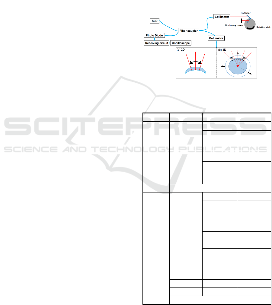
measured signal is high. Figure 1 shows a schematic

diagram of this system. In addition, Table 1 shows the

specifications of 2D and 3D system, respectively. The

2D’s super luminescent diode (SLD) light is 1310nm.

This is to measure the lens itself. In contrast, for 3D,

SLD light 856nm was selected in consideration of the

development of eyeball model for axial length

measurement.

Figure 1: A schematic diagram for TD-OCT system. (a) is

2D and (b) is 3D.

Table 1: Specifications of TD-OCT measurement system.

Algorithm Parts Item Specifications

SLD

Wavelength

1310 nm

Spectral

Width

55 nm

Resolution

13.8 μm

Measurement

stage

Position

Accuracy

1 μm

Rotation 15 scan/s

(900rpm)

Rotation

Radius

15 mm

N.A.

0.14

SLD

Wavelength

856nm

Spectral

Width

32.1nm

Resolution

10.1μm

MEMS

Angular

resolution

< 5 μrad

Maximum

scanning

angle

±10 deg

Drive

frequency

< 450 Hz

Drive voltage

-5 ~ 5 V

Cylindrical

Lens

Focal length 200 mm

Lens1

Focal length

100 mm

Lens2

Focal length

40 mm

N.A

0.015

PHOTOPTICS 2021 - 9th International Conference on Photonics, Optics and Laser Technology

2.2 2D Shape Measurement Algorithm

In this study, we propose a measurement algorithm

which makes the incidence light always hits

perpendicularly to front and back surfaces of a

spherical CL to measure its real shapes. Figure 2

shows the measurement algorithm using the metal

ball. The sample stage mechanism was designed so

that its translation movement and vertical rotation can

be changed in order to measure both front and back

surfaces’ interference echoes, which assume sign of

the vertical incidence. In the Fig. 2, the dash line

shows the initial position of the metal ball and the

solid line shows the position where it is rotated on the

vertical rotation angle and translated to get the

vertically incidence position. The position of 2

interference point (IP) is calculated by using the

vertical rotation angle and translation.

The measurement data includes the translation

distance d, the vertical rotation angle θ and the optical

path positions of the front surface interference time

𝑡



, and the back surface interference time 𝑡



. The

OCT interference times are converted into the

distance using the reflector rotation speed. Then the

distance is converted into the coordinates with the

equation (1) - (4) using the vertical rotation angle and

translation distance on this algorithm. In the case of

CLs, two interference signals occur. The interval

between them indicates the thickness. Since light

passes through the substance, the group refractive

index was taken into consideration for calculating the

back surface coordinates. Equation (1) and (2) were

used to calculate the front curvature coordinate, and

(3) and (4) were used to calculate the back curvature

coordinate.

𝑥



=dcosθ− a

(



−t



)

sinθ (1)

𝑦



=dsinθ+a

(



−t



)

cosθ − e (2)

𝑥



= dcosθ − a{t



−[t



+(t



−t



)/n]}sinθ (3)

𝑦



=dsinθ+a{t



−[t



+(t



−t



)/n]}cosθ − e

(4)

a is a time-distance conversion coefficient which

is calculated from the change of the optical path

length depending on the rotation speed of the

reflector. 𝑡



is the optical path length (time unit)

from the OCT measurement range origin to the center

of CL rotation. n is the group refractive index of the

CL. e is the difference in length between the center of

the curvature radius and the center of the CL rotation.

It was calculated by using a curvature radius of a

known spherical metal ball. Then, the curvature

radius was estimated from the (x,y) coordinates by a

circle approximation using the least-squares method.

For comparison with a conventional measurement

device, a confocal laser microscope (Sensofar: Plu

Apex) was adopted. Since it is single-sided shape

measurement device, the CL was turned over to

measure the shape of the back surface after measuring

the front surface. The curvature radius was compared

with the OCT result.

Figure 2: 2D measurement algorithm using the metal ball.

2.3 3D Shape Measurement Algorithm

In 3D algorithm, we conducted a basic experiment

using some special lenses in order to develop a non-

cylindrical lens measurement. In order to realize this

algorithm, it was designed to conduct circular

scanning by driving two MEMS mirror (Hamamatsu

Photonics: 2D-OSE201) on the vertical and

horizontal axes with a phase difference of 90 ° .

Moreover, since this MEMS mirrors don’t have a

resonance frequency, the drive frequency can be

changed, and the measurement angle can also be

changed by the drive voltage. By using two MEMS

mirrors, a cylindrical lens was used to correct the

misalignment for each axis. The number of

measurement points in this OCT system depends on

the difference between the reflector rotation

frequency 𝑓



of the variable optical path mechanism

and the drive frequency 𝑓



of MEMS mirrors.

Assuming that the minimum measurement point is 2n

(n=1, 2, 3,⋯), 𝑓



is calculated from equation (5)

using 𝑓



𝑓











𝑓



(5)

In this measurement, firstly, the time difference

𝑡



between the trigger signal at focal position of the

measurement probe and the OCT interference

position was measured. And in the circular sannning,

2D and 3D Measurement Algorithms for Real Front and Back Curved Surfaces of Contact Lenses

the time difference 𝑡





is measured. Using these time

differences, the distance r from the focal point of the

measurement probe to each measurement point is

estimated. In addition, in the MEMS mirrors, the time

difference 𝑡



and 𝑡



between the driving singnals of

MEMS mirror in the horizontal/vertical direction and

the interference positions are defined, respectively.

The incident angle θ and the vertical incident angle φ

are calculated using 𝑡



and 𝑡



. Three-dimensional

coordinates (x, y, z) are caluculated from r, θ and φ

using equation (6) – (8).

x = rcos𝜃 cos𝜑 (6)

y = rcos𝜃sin𝜑 (7)

z=rsin𝜃 (8)

After the coordinate conversion, the position (x, y,

z) of each OCT inteference point were fitted by the

least squares method of the sphere. Then, after

applying the correction, the curvature radius and

center coordinates were evaluated.

Figure 3: 3D measurement algorithm.

2.4 Measurement Sample

Rigid CLs were adopted as transparent samples. They

were practically designed and specially manufactured

for the purpose of this study. The refractive index of

the material is 1.455

± 0.02, which was measured with

Abbe’s refractometer (Atago: NAR-1T SOLID). The

curvature radii of both front and back surfaces were

manually measured with a contact gauge (NEITZ:

CGX-3). A typical CL structure including names of

each part is shown in Fig 4.

In 2D experiment, the optical lens power of 21

lenses are from -10D and 10D in 1D steps, which

were named A through U. They have the same

diameter and curvature radius of the back surface, but

the curvature radius of the front surface depends on

the lens power. Also, the curvature radius of the lens

periphery of the front surface, the diameter of the

optical zone, which is the area displaying the required

correction lens power, and the center thickness are

different depending on lens. Therefore, the

measurement range is calculated from the optical

zone diameter and the curvature radius of the front

surface.

In 3D experiment, we adopted 5 lenses which

have the specialized characteristics. It is whether the

centers of curvature radius on the front and back

surface are same or not. Accordingly, the thicknesses

are adjusted. The specifications of the sample lenses

are shown in Table 2.

Figure 4: Structure of a typical contact lens.

Table 2: Specifications of the sample lenses for 3D

measurement.

Sample

lens

Front

Surface

Curvature

Radius

Back

Surface

Curvature

Radius

Lens

Diameter

Center

Thickness

[mm] [mm] [mm] [mm]

A 7.92 7.82 10.0 0.10

B 7.97 7.82 10.0 0.15

C 7.92 6.67 10.0 1.25

D 6.77 6.67 10.0 0.10

E 7.92 6.67 10.0 0.054

3 EXPERIMENTAL RESULTS

3.1 2D Shape Measurement

In 2D measurement study, shape, curvature radius

and thickness of sphere lenses were evaluated. Figure

5 shows (a) design drawing of the lens as a

representative sample and (b) its measurement

results. In Fig. 5 (a), within 5.77 mm of the optical

zone, the curvature radius was 6.68 mm (Designed

FS1) whereas in the peripheral part, it was 7.20 mm

(Designed FS2). The curvature radius of the back

surface had a constant 6.67 mm (Designed BS). In

Fig. 5 (b), 3 trial measurements were conducted in the

vertical rotation angle, ranging from -35° to 35° in 5°

steps. Compared with the design value in Fig. 5 (a),

the same transition of the curvature radii was

observed in the OCT measurement results in Fig. 5

(b). That is, Designed FS1 and FS2 well matched with

the result (FS) 1-3 on optical zone and peripheral part,

PHOTOPTICS 2021 - 9th International Conference on Photonics, Optics and Laser Technology

Figure 5: (a) Drawing for lens design and (b) measurement

results of the front and back surfaces with OCT of sample

lens K (Power 0.00D).

respectively. When the curvature radius was

estimated by the circle approximation of the OCT

results, the curvature radii of the back surface was

6.71 mm, and for the optical zone and peripheral part

of the front surface, they were 6.70 mm and 7.21 mm,

respectively.

Figure 6 shows the result of the thickness

distribution compared with the designed values. The

thickness is shown at each vertical rotation angle,

which ranges from -30° to 30° in 1° steps. The root

mean square error (RMSE) was 5.33 μm against the

distribution of the designed thickness. The ISO

standard is only applicable to the central part and the

tolerance limit for the design value is within ±

0.02mm. Even though the experimental error of 5.33

μm takes into account the thickness of the peripheral

part, it was remarkably small compared with the

criteria value.

The curvature radius estimated by our OCT was

evaluated in comparison with Plu Apex. Figure 7

shows the measured curvature radius results of 21

sample lenses. Compared with the designed values,

with respect to the front surface, the errors from the

designed values tend to increase as the curvature radii

become large in both of our OCT and Plu Apex

results.

In our OCT results, the error is large in the sample

lens U, which has the largest difference in the

curvature radii between the front and back surfaces.

That is, since there is a big difference of incident

angles on both surfaces, the intensity of the vertically

reflected light measured within N.A. is weaker than

that of a lens with smaller difference in curvature

radius. Thus, this algorithm affects the measurement

results of the curvature radius because it determines

the measurement point based on the interference

intensity ratio between the front and back surfaces.

On the back surface, both devices caused large errors

on the same lens and their tendencies were opposite.

Figure 6: Thickness distribution of sample lens N (Power -

3.00D).

Figure 7: Estimation of curvature radii from our OCT and

Plu Apex for sample lenses.

easuring the back surface shape, the lens was turned

over to measure the front surface shape. On the other

hand, our OCT can simultaneously measure front and

back surfaces.

Here, analysis of results of Plu Apex and our OCT

was performed by using Bland-Altman analysis.

Regarding the front surface, the 95% limits of

agreement (LoA) was from -0.77% to -2.09% and the

correlation coefficient was 0.57, indicating a

proportional bias. And Plu Apex and the developed

OCT were compatible with each other on the front

surface results. On the other hand, regarding the back

surface, the error was large in the sample H to J, L

and M, but there was no systematic bias (LoA was

from -2.22% to -4.37%). Since there was no

systematic bias, the Minimal Detectable Change

(MDC) was 0.178 mm with 95% confidence interval

(CI) due to the random error. Therefore, if the error is

within 0.178 mm, the result is a measurement error. It

is large for inspection of contact lens. This mainly

came in the sample H to J, L and M results. Since CLs

are manufactured with contact gauge check, if the

measurement position is compatible with the

designed values, the measured lens is considered as a

good product. That is, there is an error factor outside

the measurement range of contact gauge. Since the

standard deviation (SD) is calculated by using the

-40 -30 -20 -10 0 10 20 30 40

Vertical rotation an

le[de

0.05

0.1

0.15

0.2

Designed thickness

Measured thickness

ABCDE FGH I JKLMNOPQRS TU

Sample lens

5.000

5.500

6.000

6.500

7.000

7.500

8.000

8.500

9.000

Designed FS

Designed BS

Measured OCT FS

Measured OCT BS

Measured PluApex FS

Measured PluApex BS

2D and 3D Measurement Algorithms for Real Front and Back Curved Surfaces of Contact Lenses

difference of the measured results from both devices,

SD became large and the MDC calculated using SD

accordingly became large. This shows that it is

possible to measure a wider range than contact gauge,

and measure the part that could not be measured by

the current method.

3.2 3D Shape Measurement

In 3D experiment, the front and back shape of CL

were simultaneously measured. The measurement

range was set to 1.53°, 3.60°, 5.66°, and 7.72° in

consideration of the optical zone where the correction

power is designed. The curvature radius and thickness

were evaluated. Table 3 shows the curvature radius of

each lens, and Table 4 shows the center coordinates,

respectively.

Regarding the front curvature radius of lens A and

lens B, lens A was 7.68 mm (error rate: 3.0%) and

lens B was 7.71 mm (error rate: 3.2%). On the other

hand, the back surface is 7.49 mm for lens A (error

rate: 4.2%) and 7.51 mm for lens B (error rate: 4.0%).

An error of about 0.3 mm was observed on the both

surfaces compared with the design values. Here, in

order to discuss the error, the simulation using known

curvature radius was performed under the same

conditions as this measurement. In other words, the

measurement environment was reproduced and the

results were evaluated. As a result, the error rate

equivalent to the measurement result by OCT was

obtained when 0.7% noise was added to the ideal

value of the sphere. And then, the error rate was

11.0% as a result of applying the correction to the

simulation data. In other words, a maximum error rate

of 11.0% can occur in this measurement environment.

Since the measurement range is narrow against the

entire sphere, the error was occurred by applying the

sphere fitting. Compared with the results, both A and

B lenses had good results in this measurement

environment. Regarding the lens C, the curvature

radius of the front surface was 8.01 mm (error rate:

1.1%), and the radius of curvature of the back surface

was 6.96 mm (error rate: 4.3%). Compared with lens

A and lens C, it had a smaller difference from the

design value on the both surfaces. Also, as the feature,

the error of the lens A is on the minus side, but the

error of the lens C is on the plus side. This was

affected by the displacement (fixing method,

humidity, etc.) due to the measurement environment.

Since the lens C has a large thickness, it is not easily

attached by deformation. Regarding the lens D, the

curvature radius of the front surface was 6.84 mm

(error rate: 1.0%), and the back surface was 6.93 mm

(error rate: 3.9%). Compared with lens A, the result

of lens D was better. Since the lens D has a smaller

curvature radius than the lens A, it is possible to

measure data in a deeper direction to the center,

which was led to good results when fitting the sphere.

Finally, the lens E had a curvature radius on the front

surface of 6.77 mm (error rate: 14.5%) and the back

surface is 6.74 mm (error rate: 1.0%). The error rate

on the lens surface was the largest. Compared with

lens C, Table 4 shows that the center coordinates of

the lens surface were shifted in the optical axis

direction, and the tendency was that they are

vertically incident on the back surface. Therefore, it

is considered that the lens E had a larger error rate on

the lens surface than the lens C, but the lens back

surface was smaller. This result suggests to

distinguish that the centers of the front and back are

same or not.

Regarding the thickness, Figure 8 shows the

thickness distribution of lens D. Since the center

coordinates of the both surfaces are the same, the

thickness is uniform. As shown in Figure 8, the

uniform thickness were obtained. Compared with the

design value, the difference was 6 μm. Also, Table 5

shows the average thickness and standard deviation

of each lens. As shown in this Table 5, accurate

measurement was possible. Regarding the lens C,

which has the largest error and standard deviation

from the design value, an error of 53 μm was occurred

because the lens thickness was set to be so thicker lens

that is not used for normal vision correction in order

to match the center coordinates of the both surfaces.

Since this lens is thick, the internal reflections

affected to the result. The thickness result verified

highly accurate measurement even when compared

with the resolution of 10.1 μm of this OCT.

Table 3: The results of each curvature radius.

Front surface[mm] Back surface[mm]

A 7.68 7.49

B 7.71 7.51

C 8.01 6.96

D 6.84 6.93

E 6.77 6.74

Table 4: The results of the center coordinates.

Front surface [mm] Back surface [mm]

x y z x y z

A 0.00 0.01 0.28 0.16 0.06 0.03

B 0.00 0.02 0.01 0.05 0.00 0.05

C 0.25 0.00 0.00 0.01 0.01 0.02

D 0.50 0.00 0.01 0.09 0.00 0.00

E 0.13 -0.01 0.01 0.08 0.00 0.00

PHOTOPTICS 2021 - 9th International Conference on Photonics, Optics and Laser Technology

Table 5: The results of the thickness.

A B C D E

Design value

[mm]

0.10 0.15 1.25 0.10 0.054

Average value

[mm]

0.088 0.143 1.197 0.094 0.055

Std [mm] 0.013 0.008 0.020 0.003 0.008

Figure 8: Lens D’s thickness distribution for each

measurement range. ‘*’ is the front surface. And ‘.’ is the

back surface.

4 CONCLUSIONS

In this paper, we proposed the 2D and 3D

measurement algorithms for the real front and back

curved surfaces of CL. Since 2D uses the interference

intensity ration of the front and back surfaces, it takes

time to measure, and although 3D has a limited

measurement range, two measurement algorithms

that can measure both shapes of transparent objects

have great advantage.

Regarding 2D measurement algorithm, changes in

curvature radius and a wide range of thickness

distributions can be measured. In recent years,

peripheral shape of CL is an important issue for the

design of new lenses, such as CL for myopia control.

The fact that OCT provides quantitative measurement

is advantageous as a CL shape measuring device.

Also, since the front and back surfaces can be

measured simultaneously, it is possible to analyze the

misalignment between the both surfaces. This is

important for small optical lenses such as CLs. For

lens curvature radius, circle approximation results

from the obtained shape coordinates were equivalent

to those of Plu Apex. Nevertheless, our OCT device

is more superior because it can measure lens front and

back surfaces simultaneously.

Regarding 3D measurement, the simulation was

performed under the same conditions and compared

with the error rate of experimental results. Compared

with the simulation data, it was confirmed that the

error rate became smaller and the accuracy was

satisfied in this measurement environment. In

addition, the thickness was sufficiently accurate

compared with the resolution of this OCT. The next

step is to evaluate toric-shaped contact lens.

From these results, 2D and 3D algorithm were

able to solve the problem of the shape measurement

device, which is the measurement of transparent

object, by measuring the front and back surfaces at

the same time. Therefore, this algorithm can be

applied to the medical field such as the

ophthalmology field. For example, it is an eyeball

shape measurement. By using this method,

information such as the corneal shape of the front and

back surfaces, thickness and the center coordinates of

the curvature radius can be obtained. Also, it can

measure non-cylindrical shapes such as keratoconus

for eye diseases in which the cornea protrudes (

Fadel 2018)

. In addition, it can be applied not only in

the medical field but also in the industrial field.

Nowadays, small lenses such as mobile phone camera

lenses is frequently used. It is also possible to

evaluate the misalignment of the front and back

surfaces, which is applicable to the inspection of such

lenses. This is an advantage of simultaneous front and

back measurement. Simultaneous measurement of the

shapes of front and back curved surfaces of

transparent bodies such as CL provides a new

measurement possibility for the industry.

REFERENCES

B. J. Coldrick, C. Richards, K. Sugden, J. S. Wolffsohn, and

T. E. Drew, “Developments in contact lens

measurement: A comparative study of industry

standard geometric inspection and optical coherence

tomography,” Contact Lens Anterior Eye, 270-276

(2016).

D. Luo, L. Qian, L. Dong, P. Shao, Z. Yue, J. Wang, B. Shi,

S. Wu, and Y. Qin, “Simultaneous measurement of

liquid surface tension and contact angle by light

reflection,” Opt. Express, Vol. 27, No. 12, 16703-

16712 (2019).

F. Drouet, C. Stolz, O. Laligant, and O. Aubreton, “3D

reconstruction of external and internal surfaces of

transparent objects from polarization state of

highlights,” Opt. Lett., 39 (10):2955-8 May (2014).

K. Saeki, D. Huyan, M. Sawada, Y. Sun, A. Nakamura, M.

Kimura, S. Kubota, K. Uno, K. Ohnuma and T. Shiina,

“Measurement algorithm for real front and back curved

surfaces of contact lenses,” Appl. Opt. 59, No. 29

(2020).

N. Tanno, S. Kishi ： “Optical Coherence Tomographic

Imaging and Clinical Diagnosis,” Medical Imaging

Technology, Volume 17: 3-10 (1990).

66.577.58

X [mm]

-1.5

-1

-0.5

0.5

1.5

1.53°

6 6.5 7 7.5 8

X [mm]

-1.5

-1

-0.5

0.5

1.5

3.60°

66.577.58

X [mm]

-1.5

-1

-0.5

0.5

1.5

5.66°

6 6.5 7 7.5 8

X [mm]

-1.5

-1

-0.5

0.5

1.5

7.72°

2D and 3D Measurement Algorithms for Real Front and Back Curved Surfaces of Contact Lenses

P. Massatsch, F. Charriere, E. Cuche, P. Marquet and C. D.

Depeursinge, “Time-domain optical coherence

tomography with digital holographic

microscopy,”Appl.Opt. 44, 1806-1812 (2005).

K. Hibino, Bozenko F. Oreb, Philip S. Fairman, and Jan

Burke, "Simultaneous measurement of surface shape

and variation in optical thickness of a transparent

parallel plate in wavelength-scanning Fizeau

interferometer," Appl. Opt. 43, 1241-1249 (2004).

H. C. Cheng and Y. C. Lin, “Simultaneous measurement of

group refractive index and thickness of optical samples

using optical coherence tomography,”Appl.Opt. 49,

790-797 (2010).

T. Shiina, Y. Moritani, M. Ito and Y. Okamura, “Long-

optical-path scanning mechanism for optical coherence

tomography,”Appl. Opt. 42, 3795-3799 (2003).

D. Fadel, “The influence of limbal and scleral shape on

scleral lens design,” Contact Lens and Anterior Eye.,

41, 321-328 (2018).

PHOTOPTICS 2021 - 9th International Conference on Photonics, Optics and Laser Technology