OptMap: Using Dense Maps for Visualizing Multidimensional

Optimization Problems

Mateus Espadoto

1,3 a

, Francisco C. M. Rodrigues

1,3 b

, Nina S. T. Hirata

1 c

and Alexandru C. Telea

2 d

Institute of Mathematics and Statistics, University of S

ao Paulo, Brazil

Department of Information and Computing Sciences, University of Utrecht, The Netherlands

Johann Bernoulli Institute, University of Groningen, The Netherlands

Keywords:

Optimization, Dimensionality Reduction, Dense Maps.

Abstract:

Operations Research is a very important discipline in many industries, and although there were many de-

velopments since its inception, to our knowledge there are no visualization tools focused on helping users

understand the decision variables’ domain space and its constraints for problems with more than two input

dimensions. In this paper, we propose OptMap, a technique that enables the visual exploration of optimization

problems using a two-dimensional dense map, regardless of the number of variables and constraints in the

problem and for any kind of single-valued objective function. We show the technique in action for several

optimization problems of different types, such as linear, nonlinear and integer, constrained and unconstrained

problems.

1 INTRODUCTION

Operations Research (OR), also called Management

Science, plays a crucial role in many industries,

from logistics to ﬁnance. Although its origins as

a discipline date from the 1950s, with the devel-

opment of the Simplex algorithm for Linear Pro-

gramming (Dantzig, 1990; Kantorovich, 1960), it is

a ﬁeld in constant development since then. The

OR practitioner has many tools at their disposal

which improve their productivity, such as alge-

braic modeling languages like GAMS (Brooke et al.,

1998), AMPL (Fourer et al., 2003) and more recently,

JuMP (Dunning et al., 2017), which enable the use of

notation very close to the mathematical deﬁnition of

optimization problems. Yet, to our knowledge, there

are no well-established visualization tools that help

understand multivariate objective functions with re-

spect to the decision variables and constraints (if any)

of the problem. Such tools are important as a com-

plement to more formal tools for getting an overall

https://orcid.org/0000-0002-1922-4309

https://orcid.org/0000-0002-0540-8510

https://orcid.org/0000-0001-9722-5764

https://orcid.org/0000-0003-0750-0502

understanding of how an objective function behaves

subject to its many parameters.

We propose a technique called OptMap, which is

an image-based visualization tool that enables the OR

practitioner to literally see the decision variables and

constraint spaces using a two-dimensional dense map,

regardless of the number of variables and constraints

in the problem. We show that OptMap can be used

in several ways, such as a debugging aid to help diag-

nose errors in the deﬁnition of constraints; as a tool to

provide insight of the optimizer’s inner workings, by

plotting the path taken from a starting point to a solu-

tion; and as a general tool to visually explore the high-

dimensional space of the decision variables in terms

of objective function value and constraint feasibility.

OptMap aims to cover the following aspects,

which, to our knowledge, are not achieved by

existing visualization techniques in the context of

optimization:

Quality (C1). We provide high-quality visualiza-

tions, that encode information at every available

screen pixel, by using a combination of dense maps,

direct, and inverse projection techniques;

Genericity (C2). We can handle many kinds of

optimization problems for single-valued objective

Espadoto, M., Rodrigues, F., Hirata, N. and Telea, A.

OptMap: Using Dense Maps for Visualizing Multidimensional Optimization Problems.

DOI: 10.5220/0010288501230132

In Proceedings of the 16th International Joint Conference on Computer Vision, Imaging and Computer Graphics Theory and Applications (VISIGRAPP 2021) - Volume 3: IVAPP, pages

123-132

ISBN: 978-989-758-488-6

123

functions. The only requirements we impose are that

the user provides implementations of the objective

function, constraints (if any), and the range for each

variable;

Simplicity (C3). Our technique is based on existing

projection techniques which have a straightforward

implementation, allowing easy replication and de-

ployment;

Ease of use (C4). Our technique has few hyperpa-

rameters, all with given presets. In most cases, users

do not have to adjust those to obtain good results;

Scalability (C5). By using a fast projection tech-

nique and caching results when possible, our method

is fast enough to allow its use during the rapid

development-test cycle of optimization models.

We structure our paper as follows. Section 2 presents

the notations used and discusses related work on visu-

alization for multivariate functions and optimization

problems, Section 3 details our method. Section 4

presents the results that support our contributions out-

lined above. Section 5 discusses our proposal. Sec-

tion 6 concludes the paper.

2 BACKGROUND

Related work concerns optimization techniques

(Sec. 2.1 and 2.2), dimensionality reduction

(Sec. 2.3), and visualization (Sec. 2.4).

2.1 Optimization: Preliminaries

Optimization problems come in many forms with re-

spect to the kind of function to be optimized, the

type of decision variables, and the existence of con-

straints. Functions are typically grouped into linear,

convex and non-convex. Linear functions are of the

form f (x) = ax +b, which deﬁnes a hyperplane; con-

vex functions can have many forms, but can be de-

ﬁned as those where the set of points above their

graph forms a convex set; non-convex functions are

neither linear nor convex (linear functions are also

convex). Decision variables can be continuous or dis-

crete: Problems with only discrete variables are called

Integer Programs (IP) (Guenin et al., 2014), whereas

problems with a combination of discrete and con-

tinuous variables are called Mixed Integer Programs

(MIP). Lastly, problems can be constrained or un-

constrained. Constraints can be characterized just as

functions (linear, convex, non-convex). Additionally,

we have box constraints, which are simple restrictions

on the variables’ domains. Problems with continuous

variables, linear objective functions, and linear con-

straints are called Linear Programs (LP). Other prob-

lems are solved by Nonlinear Programming (NLP)

techniques.

In any case, real-world optimization problems

typically have many variables and constraints. With-

out visual aids, the user typically has to rely on nu-

merical analysis to understand if the problem is mod-

eled correctly and if the results make sense. In our

opinion, having a visualization tool greatly expands

the possibilities of model analysis and debugging,

giving the user a quick way to check, for example,

if constraints are correctly deﬁned, i.e., not under- or

over-constraining by mistake, or, in the case of NLP

problems, to check how stable are the optima found,

i.e., how close they are to peaks or troughs in the data.

2.2 Optimization: Technicalities

We next deﬁne a few notations for optimization prob-

lems. Let f : R

→ R be some function to be min-

imized. Let x = (x

, . . . , x

), x

, 1 ≤ i ≤ n, be an n-

dimensional vector of n decision variables x

. Deci-

sion variables can be any combination of discrete (Z)

and continuous (R). Let O be the optimization prob-

lem described as

minimize f (x)

subject to x ∈ S

(1)

where S is the feasible set of all points that can be con-

sidered as valid for the optimization problem. For un-

constrained problems, S is R

. For constrained prob-

lems there is a set of K constraint functions c

(x) ∈

{0, 1}, k ∈ 1, ..., K, where 0 means that the point x is

infeasible with respect to the constraint c

. That is,

for constrained problems, the feasible set is deﬁned

as S = {x :

∏

(x) = 1, k ∈ 1, ..., K}.

Solvers are algorithms that ﬁnd one of several (ap-

proximate) solutions to a problem O. To do this efﬁ-

ciently, solvers use the characteristics of the problem,

such as the type of decision variables, objective func-

tion and constraints, and employ adequate heuristics

to avoid exploring all possible x ∈ S, which would be

impractical in most cases. Probably the most popular

solver algorithm is the Simplex (Dantzig, 1990; Kan-

torovich, 1960), used for linear problems and imple-

mented by software such as Clp (Forrest et al., 2020a),

Cbc (Forrest et al., 2020b) and GLPK (Makhorin,

2008). For non-linear optimization problems there are

other algorithms such as Gradient Descent, Nelder-

Mead (Nelder and Mead, 1965) and L-BFGS (Liu

and Nocedal, 1989), to name a few. Many solvers

IVAPP 2021 - 12th International Conference on Information Visualization Theory and Applications

124

work iteratively, i.e., start from a given point x

and

evolve this point until sufﬁciently close to the solution

of O.

A solution is an n-dimensional point found by

the solver which meets the criteria of being feasible

(x ∈ S) and optimal. The deﬁnition of optimality de-

pends on the type of problem and solver used: For

linear functions with linear constraints, solvers are

guaranteed to ﬁnd a global optimum solution, which

means that no other n-dimensional point provides a

lower value for the objective function f , given those

constraints. For non-linear functions, solvers may re-

turn different local optima, depending on the starting

point x

used and the shape of the objective function.

Lastly, a solver may provide the user with a

trace, or path to solution, which is the set of all n-

dimensional points where it evaluated the objective

function, starting from x

and ending with the solu-

tion, if one was found, else ending with the last point

evaluated by the solver.

2.3 Dimensionality Reduction

Dimensionality reduction (DR) is an area of research

concerned with representation of high-dimensional

data by a low number of dimensions, enabling dif-

ferent tasks to be performed on the data, such as vi-

sual exploration (Espadoto et al., 2019a). Probably

the best known DR method is Principal Component

Analysis (Jolliffe, 1986) (PCA), which has been used

in several areas for many decades. It is a very simple

algorithm with theoretical grounding in linear alge-

bra. PCA is commonly used as preprocessing step for

automatic DR on high-dimensional datasets prior to

selecting a more speciﬁc DR method for visual ex-

ploration (Nonato and Aupetit, 2018).

There are many families of DR methods,

such as Manifold Learners, Spring Embedders and

Stochastic Neighborhood Embedding (SNE) tech-

niques, among others. Manifold Learners such as

MDS (Torgerson, 1958), Isomap (Tenenbaum et al.,

2000), LLE (Roweis and Saul, 2000) and more re-

cently UMAP (McInnes and Healy, 2018) try to re-

produce in 2D the high-dimensional manifold on

which data is embedded, to capture nonlinear struc-

ture in the data. Spring Embedders, also called force-

directed techniques, such as LAMP (Joia et al., 2011)

and LSP (Paulovich et al., 2008), are popular in the

visualization literature and have a long history, with

uses other than dimensionality reduction, such as

graph drawing. The SNE family of methods appeared

in the 2000’s, and has t-SNE (Maaten and Hinton,

2008) as its most popular member. SNE-class meth-

ods produce visualizations with good cluster sepa-

ration. For extensive reviews of DR methods, and

their quality features we refer to (Nonato and Aupetit,

2018; Espadoto et al., 2019a).

We next describe the notation for DR used in the

paper. Let D = {x

}, 1 ≤ i ≤ N be a dataset of N

points x with n dimensions each. A dimensionality

reduction, or projection, technique is a function

P : R

→ R

where q  n, and typically q = 2. The projection P(x)

of a sample x ∈ D is a point p ∈ R

. Projecting a set

D yields thus a qD scatter plot, denoted next as P(D).

The inverse of P, denoted P

−1

(p), maps a point in

to a high-dimensional point x ∈ R

, aiming to sat-

isfy that P

−1

(P(x)) = x. Methods computing inverse

projections include iLAMP (Amorim et al., 2012) and

NNInv (Espadoto et al., 2019b).

2.4 Visualization

Visualization of high-dimensional data is an active

topic for several decades, with many types of meth-

ods being proposed (Buja et al., 1996; Liu et al., 2015)

and analyzed via several quality metrics (Bertini et al.,

2011). Our scope is narrower – we are interested in vi-

sualizing multidimensional functions, and more par-

ticularly, optimization processes for such functions.

The visualization of 2D functions f : R

→ R

is usually done by means of 3D height plots, con-

tour plots, or color (heatmap) plots. For functions

f : R

→ R with more than two variables (n > 2),

there are far fewer options, with Hyperslice (van Wijk

and van Liere, 1993) being a notable one. Hyperslice

presents a multidimensional function as a matrix of

orthogonal two-dimensional slices, each showing the

restriction of f to one of the 2D subspaces in R

, us-

ing the 2D function plotting outlined earlier (contour

plots, color plots, 3D height plots).

Visualizing constrained optimization problems is

similar to the above, since not only the function

has to be visualized but constraint feasibility as

well. Most techniques used for this are based on

overlaying contour plots with constraint information,

with one case where image-based techniques are

used (Wicklin, 2018). Still, such techniques cannot

work with more than two dimensions (n > 2).

The authors of iLAMP (Amorim et al., 2012) used

direct and inverse projection techniques applied to

non-linear optimization problems, to help users inter-

actively identify good starting points for optimization

problems. However, iLAMP is computationally ex-

pensive, and has quite a number of free parameters the

user needs to set. The NNInv method (Espadoto et al.,

2019b) accelerates inverse projections by over two or-

ders of magnitude as compared to iLAMP by deep

OptMap: Using Dense Maps for Visualizing Multidimensional Optimization Problems

125

learning the inverse projection function P

−1

. The

same deep learning idea was also used to accelerate

the direct projection P by Neural Network Projections

(NNP) (Espadoto et al., 2020). Recently, NNInv was

used by an image-based (dense map) technique to vi-

sualize the decision boundaries for Machine Learning

classiﬁers (Rodrigues et al., 2019), for problems with

arbitrary dimension. Their method can be conceptu-

ally seen as the visualization of a function f : R

→ C,

where f is a classiﬁer for nD data and C is a class

(label) set. We share the idea of using a dense pixel

map to visualize high-dimensional functions with this

work. However, we treat real-valued functions f

rather than classiﬁers; and our aim is understanding

optimization problems rather than understanding the

output of a classiﬁer, so we treat a different problem

and use-case.

3 METHOD

We next describe the OptMap technique. Figure 1

shows a high-level diagram of OptMap, with each

step described in detail next.

Grid-like Sample

2. Create uniform sample

DR with PCA

Phase 1: Create Mappings between Spaces

2D → nD

Phase 2: Create Visualization

1. Define variable’s domains

1. Start with

blank image

2. Sample points in 2D

and inverse project

3. Train projectors

3. Color points based

on nD projected points

Lightness

Hue

4. Draw path to solution

Evaluate

Project path

Figure 1: OptMap Pipeline.

1. Deﬁne Variable Ranges. the user speciﬁes

the domain of each variable x

for f (x

, . . . , x

When the range is the entire real axis R, we suggest

selecting a reasonable ﬁnite range to avoid having a

too coarse sampling for that variable;

2. Sample Data. We uniformly sample the ranges de-

ﬁned above for each variable, yielding a regular sam-

ple grid G

⊂ R

. We constrain the maximum number

of sample points N

max

to avoid combinatorial explo-

sion. In this paper, we used N

max

= 5M for all exper-

iments. We evaluate f on G

and call the resulting

dataset D.

3. Create Mappings. we use PCA (Jolliffe, 1986)

trained on D to create the mappings P and P

−1

from

to R

, and from R

to R

respectively.

4. Create a 2D Grid. We create an uniform grid

⊂ R

similar to G

. Simply put, G

is a pixel

image of some ﬁxed resolution (set to 800

for the

experiments in this paper). Next, we use the trained

−1

to map each grid point (pixel) p ∈ G

to a

high-dimensional point x ∈ R

. Finally, we evaluate

the objective function f (x) and optional constraints.

5. Color Pixels. We color all pixels p ∈ G

by the

values of f (P

−1

(p)), using a continuous color map,

set in this paper to the Viridis color map (Hunter,

2007). Additionally, we set the luminance of p to

reﬂect f (P

−1

(p))’s membership of the constraint-set

S, thereby indicating constraint feasibility. Note that,

strictly speaking, this colormap also has a luminance

component. Hence, luminance is actually encoding

both f and the constraints. If desired, one can easily

select to use other – more (perceptually) isoluminant

colormaps. We leave the question of what the optimal

colormap is open as part of future work.

6. Draw Path to Solution. if the solver provides the

trace to a solution, as deﬁned in Section 2.1, we can

draw it in the 2D grid by projecting them using P.

4 RESULTS

We next present several experiments that show how

our OptMap technique performs in different sce-

narios. First, we use OptMap to visualize high-

dimensional functions that have a known shape

(Sec. 4.1). Since we know the ground truth, we

can check how OptMap performs. Next, we test our

method on several unconstrained and constrained op-

timization problems (Secs. 4.2 and 4.3 respectively)

and show the added value OptMap provides in these

actual use cases.

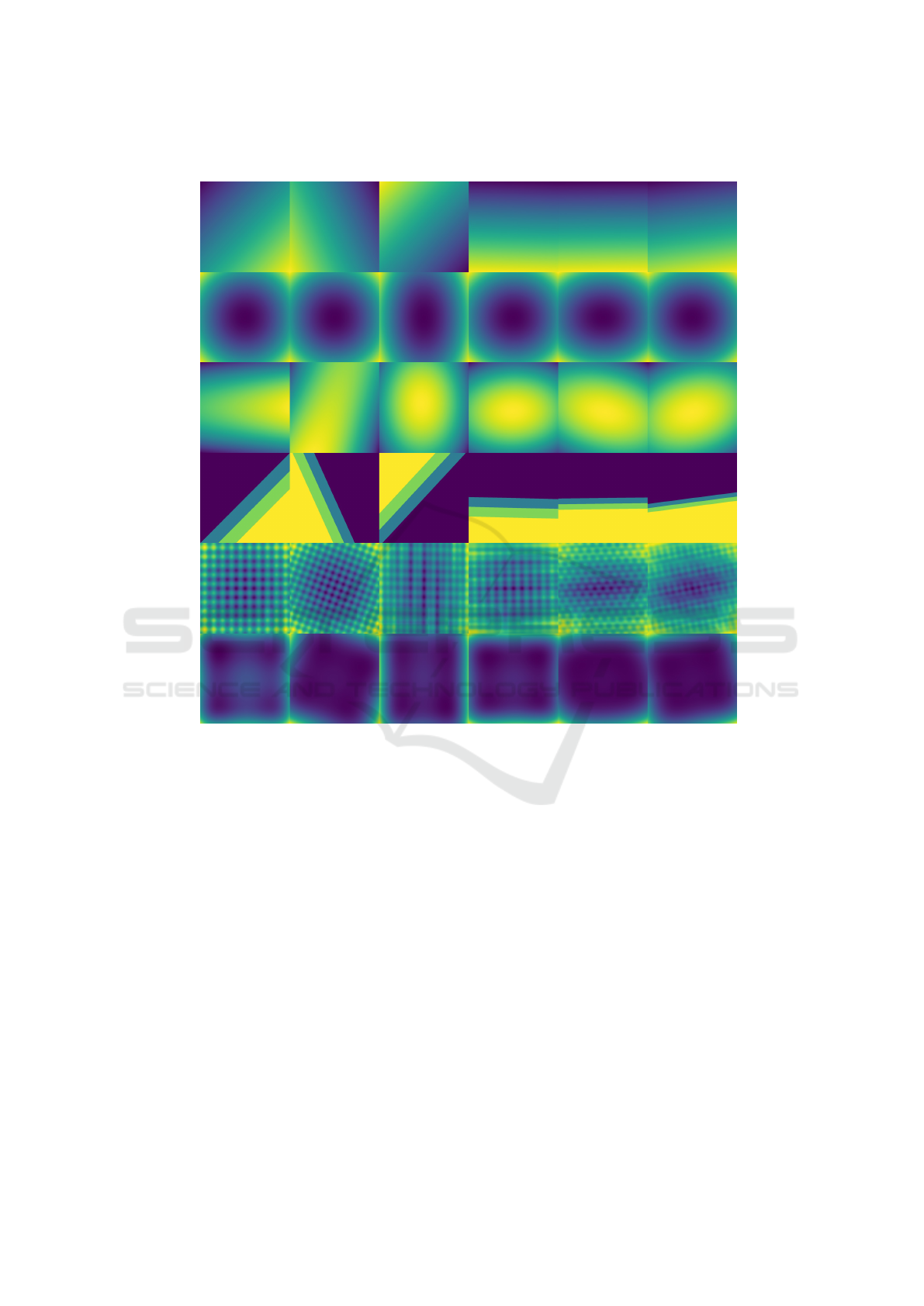
4.1 Ground-truth Functions

We use the six functions f listed in Table 1 to test

OptMap. The corresponding dense maps, computed

as explained in Sec. 3, are shown in Fig. 2. In all

cases, the domain used for all variables was x

∈

[−5, 5]. All these functions have a predictable shape

and also generalize to many dimensions. We created

dense maps using increasing numbers of dimensions

n ∈ {2, 3, 5, 7, 10, 20}. The dense map for n = 2 was

IVAPP 2021 - 12th International Conference on Information Visualization Theory and Applications

126

Dimensions (n)

2 3 5 7 10 20

Styblinski-Tang Rastrigin Step Rosenbrock Sphere Linear

Figure 2: Dense maps for functions with known shape as deﬁned in Table 1, with increasing dimensionality n > 2. Compare

these with the ground-truth maps for n = 2.

created for reference only, without using OptMap. In-

deed, for n = 2, we can directly visualize f , e.g.,

by color coding, similar to (van Wijk and van Liere,

1993). Showing these maps for n = 2 is however very

useful. Indeed, (1) for n = 2, we can show f directly,

without any approximation implied by OptMap; and

(2) given the functions’ expressions (Tab. 1), we know

that they behave similarly regardless of n. Hence,

if for n > 2 OptMap produces images similar to the

ground truth ones for n = 2, we know that OptMap

works well. And indeed, Fig. 2 shows us exactly this

– the OptMap images for n > 2 are very similar to

the ground-truth ones for n = 2. The differences im-

ply some distortion and rotations, which, we argue,

are expected and reasonably small, given the inherent

information loss when mapping a nD phenomenon to

2D.

4.2 Unconstrained Problems

We next use OptMap to show how different solvers

perform when solving different unconstrained prob-

lems (that is, variants of Equation 1). For this, we

select a subset of the functions deﬁned in Table 1,

namely Styblinski-Tang, Rastrigin and Sphere func-

tions, with varying dimensionality n. We use the

solvers listed in Table 2, grouped by solver type,

namely whether it is gradient-free or if it requires a

gradient or a Hessian. In Figure 3 we use OptMap to

show the trace provided by each solver, i.e., all the

points evaluated by the solver to get to the solution.

We see that for a simple function with a global opti-

mum (Sphere) most solvers ﬁnd an optimal solution,

except for the gradient-free methods, which seem to

struggle with the high-dimensionality of the problem

(n = 20 dimensions). For the Styblinski-Tang func-

tion, we see different but close optima were found

OptMap: Using Dense Maps for Visualizing Multidimensional Optimization Problems

127

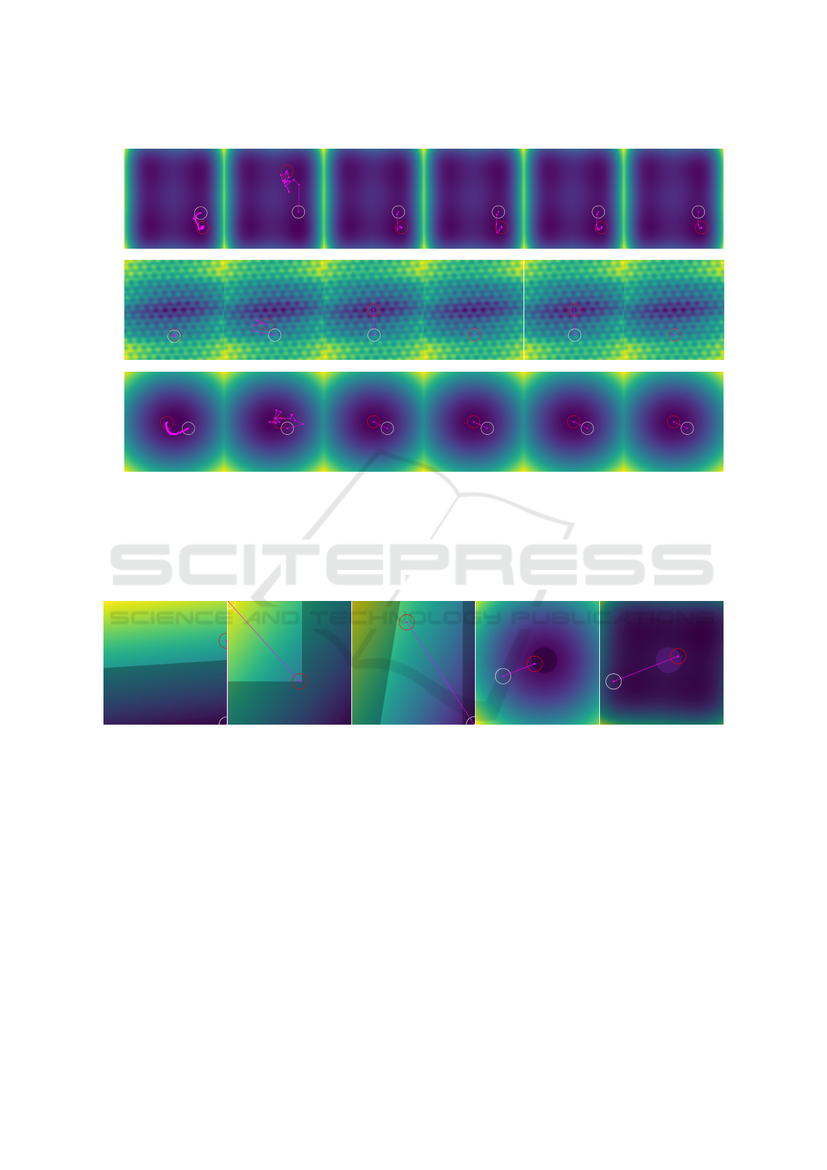
Nelder-Mead Simulated Annealing Gradient Descent Conjugated Gradient L-BGFS Newton

Rastrigin

10 dimensions

8.954 6.605 0.0 8.954 0.0 8.954

Sphere

20 dimensions

4.465 1.170 0.0 7.30e-30 0.0 5.08e-31

-167.557 -164.092 -181.694 -181.694 -181.694 -167.557

Styblinski-Tang

5 dimensions

Figure 3: Dense maps created with OptMap for unconstrained problems using the solvers deﬁned in Table 2 and some of the

functions deﬁned in Table 1. White circles indicate starting points (random vectors in 5, 10 and 20 dimensions respectively).

Red circles indicate optimal points found by the solver. The magenta lines and points show each point evaluated by the solver

to get to the solution. The numbers below each image indicate the value of the objective function at the solution; red values

indicate that the solver failed to ﬁnd an optimal solution (converge). In those cases, we list the value the solver stopped at

before aborting.

Diet Schedule Knapsack Sphere Styblinski-Tang

LP, Min, 4 vars, GLPK LP, Max, 6 vars, Clp IP, Max, 7 vars, Cbc NLP, Min, 10 vars, Ipopt NLP, Min, 10 vars, Ipopt

Figure 4: Dense maps created with OptMap for the constrained problems deﬁned in Table 3. White circles indicate starting

points (zero vector). Red circles indicate optimal points found by the solver. Magenta lines show the path from the starting

point to the solution, and darker areas indicate unfeasible regions. The texts below each image indicate type of problem,

direction (minimization or maximization), number of variables, and solver used.

by most solvers. We also see that both gradient-free

methods evaluated many more points than the other

methods, but that Nelder-Mead kept moving in the

right direction. For the same problem, Simulated An-

nealing had problems converging to an optimal solu-

tion and eventually gave up. For the Rastrigin func-

tion, which has many optima, we see that only Gra-

dient Descent and L-BFGS managed to ﬁnd the solu-

tion in a straightforward way, while the other methods

converged to the wrong solution or did not converge.

4.3 Constrained Problems

We next show how our OptMap performs when deal-

ing with constrained optimization problems – that is,

ﬁnding the minimum of some n-dimensional func-

tion f whose variables are constrained as described in

Sec. 2.1. Table 3 shows the deﬁnition of constrained

problems (objective functions and constraints) we

used. The ﬁrst three problems used are very common

in the optimization literature (Guenin et al., 2014).

The last two problems use the same Sphere and

IVAPP 2021 - 12th International Conference on Information Visualization Theory and Applications

128

Table 1: Deﬁnition of n-dimensional selected functions for

ground-truth testing.

Function Name Deﬁnition

Linear f (x) =

∑

i=1

Sphere f (x) =

∑

i=1

Rosenbrock

f (x) =

n−1

∑

i=1

100



i+1

− x



+ (1 − x

)

(Rosenbrock, 1960)

Step

f (x) =











∑

i=1

< 0

∑

i=1

< 2

∑

i=1

< 4

5 otherwise

Rastrigin f (x) = An +

∑

i=1



− A cos(2πx

)



(Rastrigin, 1974) where: A = 10

Styblinski-Tang

f (x) =

∑

i=1

−16x

+5x

(Styblinski and Tang, 1990)

Table 2: Solvers used for unconstrained problems.

Solver Type Solver

Gradient-free

Nelder-Mead (Nelder and Mead, 1965)

Simulated Annealing

Gradient required

Gradient Descent

Conjugated Gradient (Hager and Zhang, 2006)

L-BFGS (Liu and Nocedal, 1989)

Hessian required Newton

Styblinski-Tang functions deﬁned earlier, but with

nonlinear constraints added to them. Figure 4 shows

how OptMap visualizes the problem space and solu-

tion for each problem. Unfortunately, the solvers used

in this experiment, namely Clp (Forrest et al., 2020a),

Cbc (Forrest et al., 2020b), GLPK (Makhorin, 2008)

and Ipopt (W

achter and Biegler, 2006) do not provide

trace information to be drawn through the algebraic

modeling language we used, JuMP (Dunning et al.,

2017), so we only draw the straight-line path from the

(randomly chosen) starting point to solution.

In Figure 4, we can see for all problems the rela-

tionship between the objective function and the con-

straints of the problem, which provides insight on

how close to boundary conditions the solutions are.

For example, in the problems Schedule, Sphere and

Styblinski-Tang, we see that the solution found is at

the boundary of one or more constraints. This is not

the case for the Diet and Knapsack problem, which in-

dicates that some tuning to the solver’s settings may

be required to obtain better results, or even some ad-

justments to the problem deﬁnition may be done, such

as the relaxation of some constraints.

Table 3: Deﬁnition of constrained optimization problems.

Name Deﬁnition

Diet

minimize 0.14x

+ 0.4x

+ 0.3x

+ 0.75x

subject to 23x

+ 171x

+ 65x

+ x

≥ 2000.0,

0.1x

+ 0.2x

+ 9.3x

≥ 30.0,

0.6x

+ 3.7x

+ 2.2x

+ 7x

≥ 200.0,

+ 30x

+ 13x

+ 5x

≥ 250.0,

, x

≥ 0.0

Schedule

maximize 300x

+ 260x

+ 220x

+ 180x

− 8y

− 6y

subject to 11x

+ 7x

+ 6x

+ 5x

≤ 700.0,

+ 6x

+ 5x

+ 4x

≤ 500.0,

+ 5x

+ 6x

− y

≤ 0.0,

+ 8x

+ 7x

+ 4x

− y

≤ 0.0,

≤ 600.0,

≤ 650.0,

, x

, y

≥ 0.0

Knapsack

maximize 60x

+ 70x

+ 40x

+ 70x

+ 20x

+ 90x

subject to x

+ x

− 4y ≥ 0.0,

+ x

+ 4y ≥ 4.0,

30x

+ 20x

+ 30x

+ 90x

+ 30x

+ 70x

≤ 2000.0,

− 10x

≤ 0.0,

, x

, y ≥ 0.0,

, x

≤ 10.0,

y ≤ 1.0,

, x

, y ∈ Z

Sphere

minimize

∑

i=1

subject to

∑

i=1

≥ 5.0

Styblinski-Tang

minimize

∑

i=1

− 16x

+ 5x

subject to

∑

i=1

≥ 5.0

4.4 Performance

OptMap’s computation time can be divided in two

phases (Fig. 1): In phase 1, most of the time is spent

while running PCA for the sampled points in the grid

to deﬁne the mapping between the nD and 2D

spaces. This is a task that has to be done only once

for a given function f and can be reused afterwards

when one changes the solver. In phase 2, most of the

time is spent evaluating the objective function f and

its constraints. To gauge OptMap’s performance, we

ran the experiments discussed in the previous sections

on a 4-core Intel Xeon E3-1240 v6 at 3.7 GHz with 64

GB RAM. Since the evaluation of functions is usually

very fast and the pixel grid G

is of limited size (800

in our experiments), phase 2 takes only a few seconds

to run on our platform. Table 4 shows the time it takes

to run PCA in phase 1 for N

max

= 5M points, where

we see that time increases very quickly with dimen-

sionality. However, since phase 1 is required to be run

OptMap: Using Dense Maps for Visualizing Multidimensional Optimization Problems

129

only once, and since it takes at most a few minutes

to run even with a high number of dimensions n (see

Tab. 4), we argue that this is not a crucial limitation of

OptMap.

Table 4: Time to project N

max

= 5M points with different

dimensionalities n using PCA.

Dimensions n Time (sec)

3 1.19

5 0.85

7 1.45

10 2.38

20 6.62

50 32.74

100 108.71

4.5 Implementation Details

We implemented OptMap in Julia (Bezanson et al.,

2017). Table 5 lists all open-source software libraries

used to build OptMap. The optimization examples

in Sec. 4 were implemented using Optim (Mogensen

and Riseth, 2018) for the unconstrained problems,

and JuMP (Dunning et al., 2017) for the constrained

problems, using the solvers Clp (Forrest et al., 2020a),

Cbc (Forrest et al., 2020b), GLPK (Makhorin, 2008),

and Ipopt (W

achter and Biegler, 2006). Our imple-

mentation, plus all code used in this experiment, are

publicly available at github.com/mespadoto/optmap.

Table 5: Software used for the evaluation.

Library Software publicly available at

Images github.com/JuliaImages/Images.jl

ColorTypes github.com/JuliaGraphics/ColorTypes.jl

ColorSchemes github.com/JuliaGraphics/ColorSchemes.jl

Luxor github.com/JuliaGraphics/Luxor.jl

CSV github.com/JuliaData/CSV.jl

DataFrames github.com/JuliaData/DataFrames.jl

MultivariateStats github.com/JuliaStats/MultivariateStats.jl

Optim github.com/JuliaNLSolvers/Optim.jl

Clp github.com/jump-dev/Clp.jl

Cbc github.com/jump-dev/Cbc.jl

GLPK github.com/jump-dev/GLPK.jl

Ipopt github.com/jump-dev/Ipopt.jl

5 DISCUSSION

We discuss next how OptMap performs with respect

to the criteria laid out in Section 1.

Quality (C1). Figures 2, 3 and 4 show examples

of the quality of the visualizations and the kind of

insight they can provide for optimization problems.

Our dense maps are pixel-accurate, in the sense that

they show actual information inferred from the nD

function f under investigation at each pixel, without

interpolation. This is in contrast with many other

dimensionality reduction methods which either show

a sparse sampling of the nD space (by means of a 2D

scatterplot), leaving the user to guess what happens

between scatterplot points; or use interpolation in

the 2D image space to ‘ﬁll’ such gaps (Martins et al.,

2014; Silva et al., 2015; van Driel et al., 2020),

which creates smooth images that may communicate

wrong insights, since we do not know the underlying

projection is continuous.

Genericity (C2). We show how our technique per-

forms for optimization problems with varying nature,

complexity, and dimensionality. We also show that

our method can be used simply for visualizing high-

dimensional, continuous, functions by a single 2D

image, in contrast to multiple images that have to be

navigated and correlated by interaction (van Wijk and

van Liere, 1993). We also show that our technique

is independent of the optimization solvers being used;

Simplicity (C3). We use PCA for direct and inverse

projections, which is a very well known, simple,

fast, and deterministic projection method. OptMap’s

complete implementation has about 250 lines of Julia

code. Note that we also experimented with other

methods for the direct projection – namely, t-SNE as

learned by NNP (Espadoto et al., 2020) – and inverse

projection – namely, NNInv (Espadoto et al., 2019b),

obtaining good results. However, for the optimization

problems presented in this paper, PCA yielded better

results (based on ground truth comparison). Since

PCA is also simpler and faster than NNP and NNInv,

we preferred it in our work.

Ease of Use (C4). Apart from the timing experiment

in Section 4.4, we executed all experiments using the

same maximum number of sample points N

max

with

good results, which shows that the technique requires

little to no tuning to work properly;

Scalability (C5). Section 4.4 shows that our method

is highly scalable with the number of sample points

and dimensions, which enables its interactive usage

during the development cycle of optimization models.

On the other hand, scalability is inherently limited

by the resolution used to create the dense grid G

. If

the number of dimensions n and the sampling rate of

each dimension become too high, the total number

of samples N becomes prohibitive. This is inherent

to the fact that we aim to capture the dense space

spanned by the variables x

, rather than the sparse

point cloud that typical DR methods take as input.

IVAPP 2021 - 12th International Conference on Information Visualization Theory and Applications

130

To alleviate this, one could (a) consider different

sampling rates for x

, based on prior knowledge on

how f depends on each of them; (b) use OptMap

interactively by ‘zooming in and out’ of different

variable ranges to explore the high-dimensional

space; or (c) use multiresolution techniques, akin to

those already present in various optimizers.

Limitations. The projected points, such as the start-

ing, trace, and solution points, are placed in the 2D

image space at approximate positions, due to the in-

herent discrete nature of the pixel grid G

. This can

cause situations such as the one in Fig. 4 (Sphere

problem), where the optimal point found by the solver

– which is obviously feasible – is placed slightly in-

side the unfeasible region, which can be misleading.

Secondly, we noticed that due to the inherently im-

perfect mapping between nD and 2D spaces, equality

constraints that compare against constants might not

be satisﬁed during the evaluation, which will make

the drawing of feasible regions fail.

A separate aspect relates to the fact that P can

map multiple different points x ∈ D to the same pixel

p ∈ G

. Hence, the color assigned to p should ide-

ally reﬂect the combination of values f (x) of all these

points x. For categorical-valued functions f , this

can be done by using voting schemes that compute

the conﬁdence of the ﬁnal coloring (Rodrigues et al.,

2019). A low-hanging fruit for future work is to (efﬁ-

ciently) extend such schemes to our real-valued func-

tions f by using aggregation strategies such as aver-

age, min, or max.

6 CONCLUSION

In this paper we presented OptMap, an image-based

visualization technique that allows the visualization

of multidimensional functions and optimization prob-

lems. OptMap exploits the idea of constructing dense

maps of high-dimensional spaces, by using direct and

inverse projections to map these spaces to a 2D im-

age space. Suitable choices for the sampling of these

spaces, as well as using efﬁcient and well-understood

direct and inverse projection implementations, make

OptMap scalable to real-world problems. We show

that OptMap performs well in different scenarios,

such as unconstrained and constrained optimization,

with many examples that demonstrate its generic-

ity and speed. Additionally, we show that OptMap

can be used for the visualization of standalone high-

dimensional functions, even when these are not part

of an optimization problem.

Several future work directions exist. First and

foremost, it is interesting to consider using more ac-

curate direct and inverse projections for construct-

ing OptMap. Secondly, we consider using OptMap

in concrete applications, and gauging its added-value

in helping engineers designing better optimization

strategies, as opposed to existing tools-of-the-trade

for the same task.

ACKNOWLEDGMENTS

This study was ﬁnanced in part by FAPESP

(2015/22308-2 and 2017/25835-9) and the

Coordenac¸

ao de Aperfeic¸oamento de Pessoal de

ıvel Superior - Brasil (CAPES) - Finance Code 001.

REFERENCES

Amorim, E., Brazil, E. V., Daniels, J., Joia, P., Nonato,

L. G., and Sousa, M. C. (2012). iLAMP: Exploring

high-dimensional spacing through backward multidi-

mensional projection. In Proc. IEEE VAST, pages 53–

62.

Bertini, E., Tatu, A., and Keim, D. (2011). Quality metrics

in high-dimensional data visualization: An overview

and systematization. IEEE TVCG, 17(12):2203–2212.

Bezanson, J., Edelman, A., Karpinski, S., and Shah, V. B.

(2017). Julia: A fresh approach to numerical comput-

ing. SIAM review, 59(1):65–98.

Brooke, A., Kendrick, D., Meeraus, A., Raman, R., and

America, U. (1998). The general algebraic modeling

system. GAMS Development Corporation, 1050.

Buja, A., Cook, D., and Swayne, D. F. (1996). Interactive

high-dimensional data visualization. Journal of Com-

putational and Graphical Statistics, 5(1):78–99.

Dantzig, G. B. (1990). Origins of the simplex method. In A

history of scientiﬁc computing, pages 141–151.

Dunning, I., Huchette, J., and Lubin, M. (2017). JuMP:

A modeling language for mathematical optimization.

SIAM Review, 59(2):295–320.

Espadoto, M., Hirata, N., and Telea, A. (2020). Deep learn-

ing multidimensional projections. J. Information Vi-

sualization. doi.org/10.1177/1473871620909485.

Espadoto, M., Martins, R. M., Kerren, A., Hirata, N. S., and

Telea, A. C. (2019a). Towards a quantitative survey of

dimension reduction techniques. IEEE TVCG. Pub-

lisher: IEEE.

Espadoto, M., Rodrigues, F. C. M., Hirata, N. S. T., Hi-

rata Jr., R., and Telea, A. C. (2019b). Deep learning in-

verse multidimensional projections. In Proc. EuroVA.

Eurographics.

Forrest, J., Vigerske, S., Ralphs, T., Hafer, L., jpfasano,

Santos, H. G., Saltzman, M., h-i gassmann, Kristjans-

son, B., and King, A. (2020a). coin-or/clp.

OptMap: Using Dense Maps for Visualizing Multidimensional Optimization Problems

131

Forrest, J., Vigerske, S., Santos, H. G., Ralphs, T., Hafer,

L., Kristjansson, B., jpfasano, Straver, E., Lubin, M.,

rlougee, jpgoncal1, h-i gassmann, and Saltzman, M.

(2020b). coin-or/cbc.

Fourer, R., Gay, D. M., and Kernighan, B. W. (2003).

AMPL. A modeling language for mathematical pro-

gramming. Thomson.

Guenin, B., K

onemann, J., and Tuncel, L. (2014). A gentle

introduction to optimization. Cambridge University

Press.

Hager, W. W. and Zhang, H. (2006). Algorithm 851:

CG DESCENT, a conjugate gradient method with

guaranteed descent. ACM Transactions on Mathemat-

ical Software (TOMS), 32(1):113–137.

Hunter, J. D. (2007). Matplotlib: A 2d graphics environ-

ment. Computing in science & engineering, 9(3):90–

95. Publisher: IEEE Computer Society.

Joia, P., Coimbra, D., Cuminato, J. A., Paulovich, F. V., and

Nonato, L. G. (2011). Local afﬁne multidimensional

projection. IEEE TVCG, 17(12):2563–2571.

Jolliffe, I. T. (1986). Principal component analysis and fac-

tor analysis. In Principal Component Analysis, pages

115–128. Springer.

Kantorovich, L. V. (1960). Mathematical methods of orga-

nizing and planning production. Management science,

6(4):366–422.

Liu, D. C. and Nocedal, J. (1989). On the limited memory

BFGS method for large scale optimization. Mathe-

matical programming, 45(1-3):503–528.

Liu, S., Maljovec, D., Wang, B., Bremer, P.-T., and

Pascucci, V. (2015). Visualizing high-dimensional

data: Advances in the past decade. IEEE TVCG,

23(3):1249–1268.

Maaten, L. v. d. and Hinton, G. (2008). Visualizing data

using t-SNE. JMLR, 9:2579–2605.

Makhorin, A. (2008). GLPK: GNU Linear Programming

Kit).

Martins, R., Coimbra, D., Minghim, R., and Telea, A.

(2014). Visual analysis of dimensionality reduction

quality for parameterized projections. Computers &

Graphics, 41:26–42. Publisher: Elsevier.

McInnes, L. and Healy, J. (2018). UMAP: Uniform man-

ifold approximation and projection for dimension re-

duction. arXiv:1802.03426v1 [stat.ML].

Mogensen, P. K. and Riseth, A. N. (2018). Optim: A math-

ematical optimization package for Julia. Journal of

Open Source Software, 3(24):615.

Nelder, J. A. and Mead, R. (1965). A simplex method

for function minimization. The computer journal,

7(4):308–313.

Nonato, L. and Aupetit, M. (2018). Multidimensional

projection for visual analytics: Linking techniques

with distortions, tasks, and layout enrichment. IEEE

TVCG.

Paulovich, F. V., Nonato, L. G., Minghim, R., and Lev-

kowitz, H. (2008). Least square projection: A fast

high-precision multidimensional projection technique

and its application to document mapping. IEEE

TVCG, 14(3):564–575.

Rastrigin, L. A. (1974). Systems of extremal control.

Nauka.

Rodrigues, F., Espadoto, M., Hirata, R., and Telea, A. C.

(2019). Constructing and visualizing high-quality

classiﬁer decision boundary maps. Information,

10(9):280.

Rosenbrock, H. (1960). An automatic method for ﬁnding

the greatest or least value of a function. The Computer

Journal, 3(3):175–184.

Roweis, S. T. and Saul, L. L. K. (2000). Nonlinear di-

mensionality reduction by locally linear embedding.

Science, 290(5500):2323–2326. Publisher: American

Association for the Advancement of Science.

Silva, R. d., Rauber, P., Martins, R., Minghim, R., and

Telea, A. C. (2015). Attribute-based visual explana-

tion of multidimensional projections. In Proc. Eu-

roVA.

Styblinski, M. and Tang, T.-S. (1990). Experiments in non-

convex optimization: stochastic approximation with

function smoothing and simulated annealing. Neural

Networks, 3(4):467–483.

Tenenbaum, J. B., Silva, V. D., and Langford, J. C. (2000).

A global geometric framework for nonlinear dimen-

sionality reduction. Science, 290(5500):2319–2323.

Publisher: American Association for the Advance-

ment of Science.

Torgerson, W. S. (1958). Theory and Methods of Scaling.

Wiley.

van Driel, D., Zhai, X., Tian, Z., and Telea, A. (2020).

Enhanced attribute-based explanations of multidimen-

sional projections. In Proc. EuroVA. Eurographics.

van Wijk, J. J. and van Liere, R. (1993). Hyperslice. In

Proc. Visualization, pages 119–125. IEEE.

achter, A. and Biegler, L. T. (2006). On the implemen-

tation of an interior-point ﬁlter line-search algorithm

for large-scale nonlinear programming. Mathematical

programming, 106(1):25–57.

Wicklin, R. (2018). Visualize the feasi-

ble region for a constrained optimization.

https://blogs.sas.com/content/iml/2018/11/07/

visualize-feasible-region-constrained-optimization.

html.

IVAPP 2021 - 12th International Conference on Information Visualization Theory and Applications

132