Convolutional Neural Networks with Fixed Weights

Tyler C. Folsom

School of STEM, University of Washington, 18115 Campus Way NE,

Mail Stop 358534, Bothell, WA 98011, U.S.A.

Keywords: Biological Vision, Deep Convolutional Neural Networks, Functional Neuroanatomy, Image Compression,

Image Understanding, Image Convolutions.

Abstract: Improved computational power has enabled artificial neural networks to achieve great success through deep

learning. However, visual classification is brittle; networks can be easily confused when a small amount of

noise is added to an image. This position paper raises the hypothesis that using all the pixels of an image is

wasteful of resources and unstable. Biological neural networks achieve greater success, and the outline of

their architecture is well understood and reviewed in this paper. It would behove deep learning network

architectures to take additional inspiration from biology to reduce the dimensionality of images and video.

Pixels strike the retina, but are convolved before they get to the brain. It has been demonstrated that a set of

five filters retains key visual information while achieving compression by an order of magnitude. This paper

presents those filters. We propose that images should be pre-processed with a fixed weight convolution that

mimics the filtering performed in the retina and primary visual cortex. Deep learning would then be applied

to the smaller filtered image.

1 INTRODUCTION

The human brain has always been compared to the

dominant technology of the time (Daugman 1990).

The brain has been likened to clockwork, the

telegraph, a telephone switchboard or a digital

computer. It is none of these things. Inspiration from

biology dates to the early years of computing

(McCulloch and Pitts 1943) (von Neuman 1945,

1958). An artificial neuron, the perceptron, was

formulated in 1958 (Rosenblatt 1958). It attracted

much interest until 1969 with the publication of

Perceptrons showing that a single layer neural

network was only capable of doing linear

classifications (Minsky and Papert 1969). The authors

noted that it would be possible to extend the

perceptron to multiple layers, but the mathematics for

error backpropagation was not available and they

conjectured that the extension would be sterile.

Ironically, the multilayer backpropogation problem

was solved in the same year, but in a different context

(Bryson and Ho, 1975).

Neural networks were reborn in the 1980s

(Hopfield 1982), (Hinton 1987) (Rumelhart and

https://orcid.org/0000-0003-3981-6886

McClelland 1986). The difficulty of visual processing

was not appreciated until a rigorous analysis of the

problem was given (Marr 1982). Neural networks

were effective in some areas, but hand-crafted

algorithms remained more effective for computer

vision until the emergence of computation systems

that can fully exploit machine learning.

Increased computation power has enabled deep

learning systems to outperform hand-crafted

algorithms in several cases. Tensor Flow and other

specialized systems have enabled neural network

systems with more than a dozen layers to perform

well in image classification, recognition and

segmentation tasks (Badrinarayanan et al, 2016)

(Rasouli 2020) (Elgendy 2020). The outputs of a

network layer may be fully connected to the next

layer, or they may be convolutional, in which outputs

from adjacent neurons are clustered. In deep learning

systems, the network weights may start from random

and be adjusted for maximum performance on a given

task. Alternatively, a network may start with weights

that work well for a specific application and be

modified to perform another task.

516

Folsom, T.

Convolutional Neural Networks with Fixed Weights.

DOI: 10.5220/0010286805160523

In Proceedings of the 16th International Joint Conference on Computer Vision, Imaging and Computer Graphics Theory and Applications (VISIGRAPP 2021) - Volume 5: VISAPP, pages

516-523

ISBN: 978-989-758-488-6

However, it is difficult to verify that a neural

network has really learned what was intended to be

taught. The usual procedure is to train a network on a

set of images, and then present it with images that it

has not seen to test whether it generalizes. A

1000x1500 colour image contains 36,000,000 bits.

Only a small fraction of the 36 million possible

images can be tested.

Introducing a small amount of noise to an image

produces an image that looks identical to a human.

However, it can cause a neural network to wildly

misclassify it. Images that are meaningless to a

human may be classified with high confidence by a

deep neural network (Szegedy et al. 2014) (Nguyen

et al. 2015). Images contain much redundant data.

Classification errors may be reduced by filtering the

image to eliminate noise and clutter.

Artificial neural networks are loosely based on the

processing in biological systems but with significant

simplifications. The mammalian visual system has

evolved successful strategies for understanding visual

information. It applies filters to the visual stimuli.

Machine vision could benefit from a closer look at

biological vision.

This paper first gives a review of some of the

signal processing techniques used in biological

systems for image understanding. It then examines

the workings of a non-pixel machine vision

algorithm. We present the filters used by this

algorithm, which appears to retain relevant image

features while discarding noise and reducing

dimensionality by an order of magnitude. It is

suggested that images be pre-processed by the filters

used by this algorithm before being input to a deep

learning system.

2 BACKGROUND: BIOLOGICAL

VISION

One of the most striking differences from biology is

that machine vision is based on pixels. Pixels never

make it out of the eye. All vision in the brain is based

on signals that have been convolved to a pixel-less

representation. When these signals reach the primary

visual cortex, they undergo a second convolution. All

visual processing appears to be based on signals that

have undergone this transformation.

We suggest that there is no need for a neural

network to relearn the basic convolutions performed

by the eye and primary visual cortex. The first one or

two convolutional layers of vision are fixed in

biological systems and have no plasticity beyond

infanthood. Using fixed weights in the initial layer

reduces the dimensionality of the image by an order

of magnitude without sacrificing useful information.

Some of the relevant points of mammalian vision

are given below

2.1 Receptive Fields

Hubel and Wiesel received the Nobel prize for

demonstrating that individual neurons in the cat retina

responded to a difference in contrast in a small

circular region of the visual field (Hubel and Wiesel,

1977). This transformation can be modelled as a

circular difference of Gaussians (DOG) or by several

other models.

There are five types of neurons in the retina,

starting with the rod and cone photoreceptors and

culminating in the ganglion cells. A receptive field of

a retinal ganglion cell is defined to be that area of the

visual field in which a change of illumination will

result in a change in the signal transmitted by the

nerve cell. Retinal receptive fields have two

antagonistic subfields. A bright spot striking the

centre may result in an increased output, while

increased illumination in the outer annular region will

result in a decreased signal. The DOG model

represents the inner region as a Gaussian with a

narrow extent and the outer region as a Gaussian with

a wider extent.

The axons of retinal ganglion cells form the optic

nerve over which visual information is transmitted to

the brain. If a receptive field has uniform contrast, it

transmits no signal. The brain gets strong signals from

areas of high contrast.

2.2 Cortical Transformations

Upon reaching the primary visual cortex (V1) the

retinal signals are again convolved to be sensitive to

oriented edges, disparity and speed (Kandel et al.,

2013). These patterns are largely invariant across

individuals and across species.

This convolution can be modelled by a Gabor

function, which is a sine wave modulated by a

circularly rotated Gaussian. A Gabor function is

shown in Figure 1. Several other models fit the data.

The receptive field corresponding to a simple

cortical cell is selective for step edges or bars. The

response will vary based on the position, orientation,

contrast, width, motion or binocular disparity of the

stimulus.

Convolutional Neural Networks with Fixed Weights

517

Figure 1: Gabor Function.

2.3 Simple and Complex Cells

Primary visual cortex contains both linear simple

cells and non-linear complex cells (Antolik and

Bednar 2011). The simple cells respond to different

phases of a sine grating, but the complex cells do not.

The complex cells are independent of the exact

position of the stimulus to which they respond. The

function of simple cells is better understood than that

of complex cells.

2.4 Retinotopic Maps

Signals that are close together in the visual field

remain close together at higher layers of brain

processing. Cells are precisely organized into

modules (Miikkulainen, 2005). Retinotopic brain

organization extends to higher levels (Gattass et al.,

2005). This idea is replicated in the layouts

commonly used for convolutional neural networks

(CNN). The strength of a signal from a neuron may

be amplified or attenuated based on lateral inhibition

or excitation from adjacent neurons (Nabet & Pinter

1991).

2.5 Image Compression

The retina has 87 million rods and 4.6 million cones

(Lamb 2015). These are processed in the eye and

leave as the axons of the ganglion cells that form the

optic nerve. The optic nerve has only 1 million fibres

(Levine, 1985).

2.6 Separate Paths

The optic nerve goes to the lateral geniculate nucleus

(LGN) of the thalamus and then travels to the primary

visual cortex (V1). At the thalamus, the signals

separate into a parvocellular path, which is largely

devoted to form, detail and colour, and a

magnocellular path, which is largely devoted to

motion. These paths remain separate through V1, V2

and V3. The parvocellular path splits off to V3a, V4

(which also receives magnocellular data) and the

Inferior Temporal area. From V3 the magnocellular

path goes to V5, Posterior Parietal, and frontal eye

fields (Kandel et al., 2013).

Cell specialization in the brain may extend to the

retina. Three different types of ganglion cells have

been identified in the cat: X, Y and W cells (Levine

& Shefner 1991). Y cells are largest and most often

encountered by electrodes, but they make up only 4%.

Like the complex cells, Y cells are nonlinear and give

a transient response to stimuli. The linear X cells

make up 55%. Both X and Y cells project to the

thalamus.

The W cells make up the remaining 41% but do

not go to the cortex of the brain. Instead, they go to

the brain stem and are thought to not be part of

conscious vision. Their role seems to be detecting the

most salient features of the image and directing

unconscious eye movements to concentrate on these

features.

2.7 Expected Input

The cells of V1 receive input from the eye. However,

they have more inputs from higher centres of the

brain, whose function appears to be making an

expected image more likely (Kandel et al. 2013).

Psychologists distinguish the sensation that is input to

the senses from the perception of what the data

represents. There appears to be a strong feedback

mechanism in which an expected model of the

phenomenon helps drive what is perceived.

2.8 Non-uniform Representation

The retinotopic organization is extremely dense at the

fovea, and less so on the periphery. The distribution

can be modelled as log-polar (Zhang, 2006). The eye

makes constant non-voluntary micro-motions

(saccades) to examine relevant areas. Spatial filtering

ensures that the visual system does not respond to

noise (Wilson et al. 1990).

2.9 Colour

Most of an image’s information is in the grey scale;

colour makes a minor contribution. Human cones are

sensitive to three wavelengths, peaking at 558

VISAPP 2021 - 16th International Conference on Computer Vision Theory and Applications

518

(yellow-green), 531 (green) and 420 nm (blue). Only

5% of the cones are sensitive to blue and the eye is

much less sensitive to an equiluminance image that

differs only in chrominance.

JPEG and MPEG image compression is largely

directed to the luminance content of the image, with

reduced emphasis on the chrominance (Rabbani

2002). Images are commonly stored in a compressed

format, but then put into a full RGB format with

redundant data before processing.

As demonstrated by Land’s famous experiment,

colour is a psychological construct, not a physical one

(Land 1985). The same wavelength of light can be

perceived as different colours.

Other species have different wavelength

sensitivity. Birds may have four different cone types.

Warm blooded animals cannot make effective use of

the infrared spectrum, but this limitation does not

apply to cold blooded animals. Ultraviolet light tends

to damage the eye and is avoided by animals. Some

insect eyes are sensitive to light polarization.

Biological restrictions do not apply to silicon

photoreceptors which tend to be sensitive to infrared.

Considerable ingenuity has been applied to circuits to

make them mimic human vision. Machine vision has

superhuman capabilities which can be exploited.

Multispectral imaging is common in satellite land

observation systems.

2.10 Early Learning

There is not enough information in the DNA to fully

specify brain connections. Animals wire their brains

in utero or in early life. Kittens raised in a visually

deprived environment never develop normal vision.

Humans take five years to reach full visual acuity

(Van Sluyters et al. 1990). However, once the

fundamental connections for the eye and primary

visual cortex has been learned, there does not appear

to be further plasticity.

2.11 Selective Cells

At higher layers of cortex in macaque monkey there

are single cells that respond strongly to a particular

feature, such as a face or hand, at any position.

(Goldstein and Brockmole, 2014). Such cells may

respond to only to faces or to hands. Some seem to

encode facial parts such as eyes or mouth. Some cells

are specific for responding to the face of an individual

monkey or human.

The digitized filter would be 7x7 less three pixels at each

corner or 37 pixels.

2.12 Shallow Computation

Cell processing speeds are on the order of a

millisecond in neurons, but a nanosecond in silicon.

Despite a million to one speed disadvantage, human

vision is superior to machine vision. This

performance is achieved through massive parallelism.

A human can perceive a visual stimulus and react to

it in less than a second. This implies that the

computational process is done in under 1000 steps.

3 PROPOSED METHOD

It is proposed that deep learning start with a fixed

convolution that mimics the signal transformations

performed by the retina and simple cells of primary

visual cortex. This reduces the dimensionality of the

image by an order of magnitude without sacrificing

relevant detail. It removes the computational burden

of needing to find weights for the initial layers. The

initial image transformation would be handled by an

overlapping hexagonal grid of receptive fields. The

size of the receptive fields can be either fixed or set

dynamically. Recommended minimum size is seven

pixels in diameter; maximum about 20 to 30.

Dynamic resizing of receptive field size is possible,

mimicking the attention to areas of high curvature

achieved by saccades. This processing is done on

monochrome images, with lower resolution

chrominance components handled by a different path.

3.1 Quadrature Disambiguation

The system hypothesizes that at the scale of interest,

the contents of a receptive field represent a straight

line at an unknown position and orientation with

uniform contrast on either side. Note that the

receptive fields are circular; not square. A receptive

field of diameter 7 covers 38 pixels (π∙3.5

);

diameter of 20 covers 340 pixels. After convolution,

either of these fields can be reduced to five numbers.

This is compression 7:1 to 68:1 for a monochrome

image, though with overlap image compression

would be about half that. A colour image would be

represented by the five monochrome filters plus two

more for colour. Without accounting for overlap,

colour image compression ranges from 16:1 to 145:1.

An algorithm called Quadrature Disambiguation

has been developed that can process these five

numbers to detect the exact orientation of the edge,

Convolutional Neural Networks with Fixed Weights

519

though the equation needs to be solved numerically

(Folsom and Pinter, 1998). Knowing the orientation,

the convolutional outputs can be steered to predict the

results of convolving with a quadrature pair of filters

exactly aligned to the image orientation. From their

phase, the edge position can be determined to sub-

pixel resolution. Edge contrast can be computed. If

the contrast is low, the receptive field is judged to

have no feature.

Having detected an edge at a particular position

and orientation, the system can compute what the

filter outputs would have been had the hypothesis

been true that the receptive field contained only an

ideal edge. The difference of the ideal filters from the

actual ones can be processed by the same algorithm

to find a secondary edge. If the residual edge has low

contrast, the receptive field feature is classified as an

edge. Otherwise, it is a corner or point of inflection.

The intersection of the two edges gives the corner

location and angle.

Steerability means that under certain

circumstances, the response of an oriented filter can

be interpolated from a small number of filters

(Adelman and Adelson, 1991). The five convolution

filters used above consist of a pair of orthogonal even

functions and three orientations of odd functions.

These have a similar appearance to filters often found

in convolutional neural networks, but have the

desirable properties of compact support, smoothness

and steerability.

Researchers have detected simple cell neurons in

V1 that are responsive to oriented edges; other cells

respond to bars. These have been called edge

detectors and bar detectors. It may be that the “bar

detectors” are the conjugate phase of an edge

detector. By looking at the phase difference of a

properly oriented edge detector and its conjugate, one

can determine the position of the edge within the

receptive field.

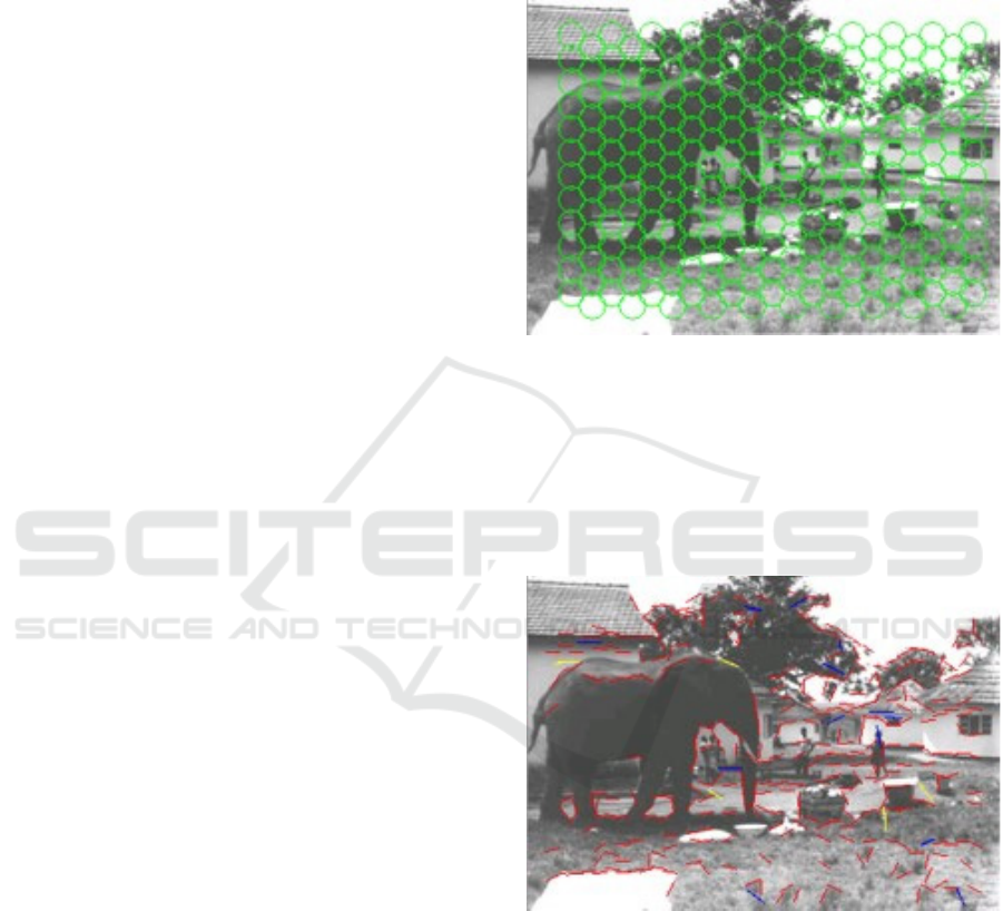
Figure 2 gives an example for a coarse tiling of an

image. It uses slightly overlapped receptive fields of

diameter 20 pixels, arranged in a 12 by 21 hexagonal

grid. Five filters at the 252 locations of the grey-scale

image means that the 83,349-pixel image has been

reduced to 1260 numbers. These numbers are then

processed to find the locations and orientations of

edges. The more prominent edges are visualized by

red and blue segments in Figure 3. It should be noted

that edge detection in image processing produces a

binary image of edge locations which requires further

processing to fit lines. By contrast, the output from

Quadrature Disambiguation is a list of edge locations,

orientations and contrast. The information could be

further processed to draw a cubic spline outlining

features. Lateral inhibition and excitation can be used

to dynamically change the contrast threshold for edge

recognition, filling in phantom lines. Grouping

edgelets together to form polylines has been done for

stereo depth perception (Folsom 2007).

Figure 2: Green circles give an image tiling.

This example is a coarse tiling leading to coarse

edge detection. Finer results can be obtained by

decreasing the diameter of the receptive fields and

increasing their overlap. Using a diameter of 12 pixels

would give a 37 by 22 grid for a total of 874 locations.

A diameter of 8 would give 1972 locations.

Figure 3: Visualization of detected edges.

It has been shown algorithmically that it is

possible to extract the key information in an image

after systematic convolution by filters with fixed

weights. Pixels are not required. This paper is not

advocating using the Quadrature Disambiguation

algorithm. Instead, it is pointing out that since the

information is contained in the convolved image, it is

discoverable by deep learning.

VISAPP 2021 - 16th International Conference on Computer Vision Theory and Applications

520

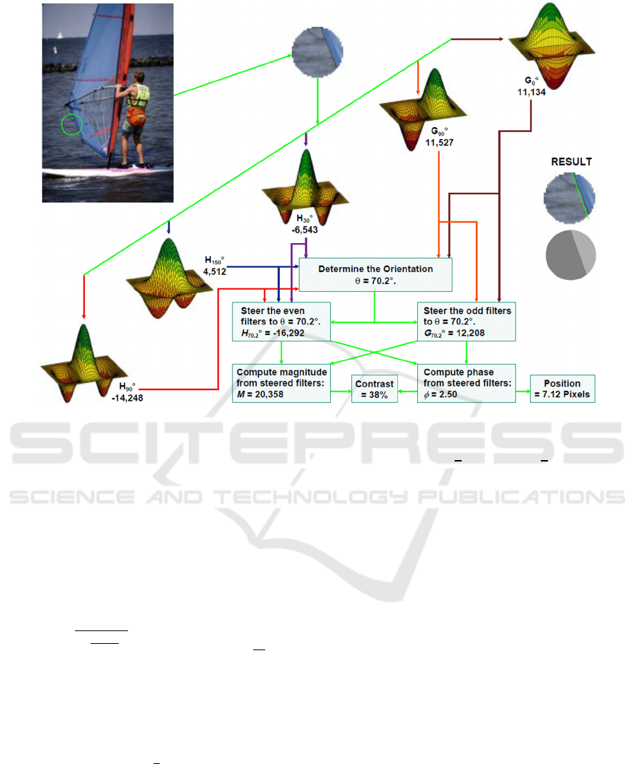
Figure 4: Filters for image simplification (Folsom and Pinter 1998).

3.2 Filters

Figure 4 illustrates how five filters can be used to find

the orientation, position and contrast of the dominant

edge in a receptive field. These filters are windowed

by a circularly symmetric function that resembles a

Gaussian but has compact support and is infinitely

differentiable. For a filter of diameter d, centred at c,

the window is given by rotating

𝑤



𝑥





⎩

⎨

⎧

1𝑓𝑜𝑟 𝑥𝑐

𝑒





















𝑓𝑜𝑟 𝑐

𝑥

𝑐





0𝑜𝑡ℎ𝑒𝑟𝑤𝑖𝑠𝑒

(1)

Outside the radius of d/2, w(x) does not exceed

0.0082, and it is zero outside a radius of 5d/8.

The even filters are set to

𝐺



𝑥



𝑤𝑥12







𝑥𝑐







 (2)

The parameter α is set to 5.665 so that the filter

gives zero response to a blank receptive field. The

two even filters are rotated to be orthogonal to each

other, resulting in the two filters G

0°

and G

90°

Odd filters are given by

𝐻



𝑥



𝑤𝑥𝛾







𝑥𝑐



𝛽





𝑥 𝑐



 (3)

Maximum phase linearity is achieved by setting

γ=2.205 and β=0.295. The three odd filters are rotated

to form H

30°

, H

90°

and H

150°

. For a colour RGB image,

these five filters would be applied to monochrome

pixels formed by (R+G+B)/3. These five numbers

would be supplemented by a red chrominance filter

produced by applying w(x) to pixels formed from

(R-G)/2 and a blue filter C

from convolving pixels

(2B-R-G)/4 with w(x).

In order to produce the fixed weights to be used

on the first stage of the convolutional neural network,

perform the following tasks:

 Select a pixel diameter.

 Arrange the receptive fields in a grid that tiles the

image.

 For the given diameter, compute the filter

coefficients G

0°

and G

90°

from equations (1) and

(2).

 Compute the filter coefficients H

30°

, H

90°

and

150°

from equations (1) and (3).

 Compute C

and C

from equation (1).

 Apply the filters to the grey-scale or coloured

pixels as appropriate.

Convolutional Neural Networks with Fixed Weights

521

 All subsequent layers of the CNN will learn

weights from these numbers and will have no

access to the original image.

A variant would be to select two or more scales

for diameters.

In summary, a circular region of an image is

reduced to the seven numbers G

0°

, G

90°

, H

30°

, H

90°

150°

, C

and C

. An overlapping circular grid

processed to extract these numbers contains the key

information that deep learning needs for image

understanding. On a colour image with diameter d set

to 9, and with 50% overlap, image compression is

13:1. For a less detailed analysis, setting d to 30 gives

compression of 150:1.

Code to implement these filters is on

https://github.com/elcano/QDED in file Features.c.

3.3 Deep Learning

The following architecture is proposed:

 The input image undergoes a fixed

convolution. Each receptive field is reduced to

five numbers, plus two additional numbers for

red-green and blue-yellow colour contrast. This

layer corresponds to V1 simple cells (V1S).

The neural network has no access to the image

feeding V1S.

 Network layers connected to the V1S input

layer should be convolutional and grouped

modularly. They may be organized into

separate paths to recognize form, motion and

colour.

 V1S may feed to V1C, which corresponds to

the ability of the complex cells to find features

over a wider range (Chen et al. 2013).

 Modules should be connected in a fashion that

allows lateral excitation or inhibition of a

feature based on its presence in neighbouring

cells (Jerath et al., 2016).

 There should be feedback from the final

classification outputs back to V1S to bias

perception in favour of the expected result.

 A shallow learning network should implement

an alphabet for visual recognition. This might

include generic faces, hands, letters or

geometric shapes. The trained network should

be included as a building block for most

models.

4 RESULTS

This is not a research paper; rather it is a position

paper arguing that CNN would benefit from an image

pre-processing step that reduces the dimensionality of

images without discarding useful information. The

technique has not been implemented in deep learning

systems. Animals have used these techniques for

millennia. Even tiny-brained creatures have

developed visual systems superior to most machine

vision systems.

5 CONCLUSIONS

Pixels are not the fundamental visual element. Fixing

the weights for the first network layer reduces its size.

Since the initial convolution has been shown to

include key image features, image sizes can be

compressed by an order of magnitude without

information loss. The reduced image size leads to

faster deep learning. Filtering produces a more stable

system with better noise immunity. It protects the

network from learning weird filters for its first stage.

It may be the solution to the problem of networks that

produce wildly different classifications for images

that look identical to humans.

REFERENCES

Daugman, J, 1990. Brain Metaphor and Brain Theory in

Computation Neuroscience. Schwartz, E. L. Editor,

MIT Press.

McCulloch, W. S., Pitts, W, 1943. “A Logical Calculus of

the Ideas Immanent in Nervous Activity”, Bulletin of

Mathematical Biophysics, pp. 115-133.

von Neumann, J. 1945, "First draft of a report on the

EDVAC," reprinted 1993 in IEEE Annals of the History

of Computing, vol. 15, no. 4, pp. 27-75.

von Neumann, J. 1958. The Computer and the Brain. Yale

University Press.

Rosenblatt, F., 1958. “The Perceptron: A Probabilistic

Model for information and Storage in the Brain”,

Psychological Review, pp. 386-408.

Minsky, M., Papert, S., 1969. Perceptrons, MIT Press.

Bryson, A. E., Ho, Y-C, 1975. Applied Optimal Control.

Taylor & Francis.

Hopfield, J. J. 1982. Neural Networks and Physical Systems

with Emergent Collective Computational Abilities.

Proceedings of the National Academy of Sciences pp

2554-2558

Hinton, G.E., 1987. Connectionist Learning Procedures.

Carnegie-Mellon University Technical Report CMU-

CS-87-115.

VISAPP 2021 - 16th International Conference on Computer Vision Theory and Applications

522

Rumelhart, R. D., McClelland, J. L. 1986. Parallel

Distributed Processing, MIT Press.

Marr, D. 1982. Vision, W. H. Freeman & Co.

Badrinarayanan, V., Kendall, A., Cipolla, R., 2016. SegNet:

A Deep Convolutional Encoder-Decoder Architecture

for Image Segmentation.

https://arxiv.org/abs/1511.00561

Rasouli, A. 2020. Deep Learning for Vision-based

Prediction: A Survey. https://arxiv.org/abs/2007.00095

Elgendy, M. 2020. Deep Learning for Vision Systems.

Manning.

Szegedy, C. et al. 2014. Intriguing Properties of Neural

Networks. https://arxiv.org/abs/1312.6199

Nguyen, A., Yosinski , J., Clune J. 2015. Deep neural

networks are easily fooled: High confidence predictions

for unrecognizable images, IEEE Conference on

Computer Vision and Pattern Recognition (CVPR),

Boston, MA, pp. 427-436.

Hubel, D. H., Wiesel, T. N., 1977. Ferrier Lecture:

Functional Architecture of the Macaque Monkey

Visual Cortex. Proceedings of the Royal Society of

London, Series B, Vol 198, pp 1-59.

Kandel, E. R., et al. 2013. Principles of Neural Science,

McGraw-Hill, 5th edition.

Levine, M. W., Shefner, J. M. 1991. Fundamentals of

Sensation and Perception. Brooks/Cole.

Antolik, J. Bednar, J. 2011. Development of Maps of

Simple and Complex Cells in the Primary Visual

Cortex, Frontiers in Computational Neuroscience, Vol

Touryan, J., Lau, B., Dan, Y., 2002. Isolation of Relevant

Visual Features from Random Stimuli for Cortical

Complex Cells. Journal of Neuroscience, 22 (24) pp.

10811-10818.

Miikkulainen, R., Bednar, J. A., Choe, Y., Sirosh, J., 2005.

Computational Maps in the Visual Cortex, Springer.

Gattass, R. et al., 2005 Cortical visual areas in monkeys:

location, topography, connections, columns, plasticity

and cortical dynamics. Philosophical. Transactions of

the Royal Society. B360709–731.

Nabet, R., Pinter, R. B. 1991. Sensory Neural Networks:

Lateral Inhibition, CRC Press.

Lamb, T. D. 2016. Why Rods and Cones? Eye 30 pp. 179-

195.

Levine, M. D., 1985. Vision in Man and Machine,

McGraw-Hill.

Zhang, A. X. J., Tay, A. L. P., Saxena, A. 2006. Vergence

Control of 2 DOF Pan-Tilt Binocular Cameras using a

Log-Polar Representation of the Visual Cortex. IEEE

International Joint Conference on Neural Network

Proceedings, Vancouver, BC, 2006, pp. 4277-4283.

Rabbani, M. 2002. JPEG2000 Image Compression

Fundamentals, Standards and Practice. Journal of

Electronic Imaging 11(2).

Wilson, H. R. et al. 1990. The Perception of Form: Retina

to Striate Cortex in Spillman, L. and Werner, J. S. (eds)

Visual Perception: The Neurophysiological

Foundations, Academic Press.

Land, E. H., 1985. Recent Advances is Retinex Theory in

Ottoson D., Zeki S. (eds) Central and Peripheral

Mechanisms of Colour Vision. Wenner-Gren Center

International Symposium Series. Palgrave Macmillan.

Van Sluyters, R. C., et al, 1990. The Development of Vision

and Visual Perception, in Visual Perception: The

Neurophysiological Foundations, Spillman, L. and

Werner, J. S., editors, Academic Press.

Goldstein, E. A., Brockmole, J. R. 2014. Sensation and

Perception, Cengage Learning, 10

Edition.

Folsom, T. C., Pinter, R. B., 1998. Primitive Features by

Steering, Quadrature, and Scale. IEEE Transactions on

Pattern Analysis and Machine Intelligence, pp. 1161-

1173.

Adelman, W. T., Adelson, E. H., 1991 The Design and Use

of Steerable Filters. IEEE Transactions on Pattern

Analysis and Machine Intelligence, Vol 13; pp 891-906.

Folsom, T. C., 2007 Non-pixel Robot Stereo, IEEE

Symposium on Computational Intelligence in Image

and Signal Processing, April 2, Honolulu, HI, pp 7 -12.

Chen, D., Yuan, Z, Zhang, G., Zheng, N., 2013.

Constructing Adaptive Complex Cells for Robust

Visual Tracking. Proceedings of the IEEE International

Conference on Computer Vision, pp. 1113-1120.

Jerath, R., Cearley, S. M., Barnes, V. A., Nixon-Shapiro, E.

2016. How Lateral Inhibition and Fast Retinogeniculo-

Cortical Oscillations Create Vision: A New Hypothesis.

Medical Hypotheses, Vol. 96, pp 20-29

Convolutional Neural Networks with Fixed Weights

523