Modeling a priori Unknown Environments:

Place Recognition with Optical Flow Fingerprints

Zachary Mueller and Sotirios Diamantas

Department of Engineering and Computer Science, Tarleton State University,

Texas A&M University System, Box T-0390, Stephenville, TX 76402, U.S.A.

Keywords:

Place Recognition, Optical Flow, Optical Flow Fingerprints, Loop Closing.

Abstract:

In this research we present a novel method for place recognition that relies on optical ﬂow ﬁngerprints of

features. We make no assumptions about the properties of features or the environment such as color, shape,

and size, as we approach the problem parsimoniously with a single camera mounted on a robot. In the training

phase of our algorithm an accurate camera model is utilized to model and simulate the optical ﬂow vector

magnitudes with respect to velocity and distance to features. A lognormal distribution function, that is the

result of this observation, is used as an input during the testing phase that is taking place with real sensors and

features extracted using Lucas-Kanade optical ﬂow algorithm. With this approach we have managed to bridge

the gap between simulation and real-world environments by transferring the output of simulated training data

sets to real testing environments. In addition, our method is highly adaptable to different types of sensors

and environments. Our algorithm is evaluated both in indoor and outdoor environments where a robot revisits

places from different poses and velocities demonstrating that modeling an unknown environment using optical

ﬂow properties is feasible yet efﬁcient.

1 INTRODUCTION

This research shows how to develop a model that es-

timates the probability of having revisited the same

place or site based on optical ﬂow patterns. In order

to accomplish this we do this in two phases, training

and testing. The training phase is solely carried out on

a simulator, drastically reducing both time and work

in the estimation process. In addition, our method is

adaptable to different types of environments as well

as camera sensors. This research shows that it is pos-

sible to train a model in a simulator and to then use the

simulated output as input during the testing phase for

real-world environments. The simulated results rely

on accurate camera calibration and motion and dis-

tance parameters between camera and features. The

training phase which is based on simulation acts com-

plementary to the training phase which is taking place

with real-world camera and robotic systems. A simi-

lar training data set has also been used in (Diamantas

et al., 2010) where results obtained using a simulation

engine only.

In the training sessions we consider only two pa-

rameters, the velocity of the robot and the distance

between the robot and the target landmark. By gener-

ating optical ﬂow patterns each time the robot is enter-

ing and leaving an area, we is able to compare and rec-

ognize areas that we have been in before, even when

entering the area from different angles or velocities.

Then, based on the training done via simulator, a sim-

ilarity score is produced. This method of re-visiting

a site is similar to the method that insects utilize in

nature when entering or exiting an area.

Place recognition has always been a fundamental

problem in robotics and computer vision. A robot

that is capable of recognizing a previously unknown

environment is in great need, as this capability is in-

terwoven with localization and mapping problems in

robotics science. Place recognition using visual infor-

mation has attracted much attention the last few years

especially since the advent of algorithms that are ro-

bust to scaling and camera orientation (Lowe, 1999),

(Bay et al., 2008b). While optical ﬂow has become

a popular topic in the last decades, there has been no

research done previously for place recognition using

optical ﬂow ﬁngerprints. Most place recognition re-

search is done using properties of the environment,

while optical ﬂow uses the property of the camera mo-

tion, and is a function of the velocity of the camera

and the distance between the camera and the object.

Mueller, Z. and Diamantas, S.

Modeling a priori Unknown Environments: Place Recognition with Optical Flow Fingerprints.

DOI: 10.5220/0010271007930800

In Proceedings of the 16th Inter national Joint Conference on Computer Vision, Imaging and Computer Graphics Theory and Applications (VISIGRAPP 2021) - Volume 5: VISAPP, pages

793-800

ISBN: 978-989-758-488-6

793

Optical ﬂow is the rate of change of image motion,

which is obtained from the motion of the autonomous

agent. In both the simulator and on the robot, the cam-

era is placed perpendicular to the direction of motion,

so a translational optic ﬂow is generated. Since the

optic ﬂow only uses two parameters, all other infor-

mation is not considered. This allows for the environ-

ment that the robot is in to be unknown and unstruc-

tured.

Previous works used a simulation to model the de-

viation of an optical ﬂow vector, using distance and

velocity (Diamantas et al., 2010; Diamantas et al.,

2011). Building upon that, our current model trains

using vector magnitudes that vary with respect to dis-

tance and velocity. When testing in the real-world en-

vironment we are using a Dr Robot 4x4 mobile robot

equipped with a Blackﬂy S USB3 camera.

Optical ﬂow is a method that is inspired by biol-

ogy, speciﬁcally by the way honeybees use optical

ﬂow for navigation and obstacle avoidance. Biolog-

ical inspiration provides solutions to common prob-

lems that robots encounter. By utilizing optical ﬂow

we gain multiple advantages. First, we gain algo-

rithmic simplicity and performance, which in turn

saves on power consumption. Second, we gain in-

sight into the biological organisms that will, in turn,

help us perceive and understand the underlying mech-

anisms that facilitate biological organisms (Diaman-

tas, 2010). The ﬁnal advantage to using optical ﬂow is

that we do not store the images used, only the optical

ﬂow patterns. This removes image retrieval times, and

processing between images is not required. This fur-

ther contributes to the time efﬁciency of this method.

This paper comprises four sections. Following is

Section 2 where work on optical ﬂow is presented. In

Section 3 the methodology of the probabilistic model

that is divided into the training phase and the testing

phase is presented. Results are also presented in this

section from experiments carried out both in indoor

and outdoor environments with the robot re-visiting

places at varying velocities and distances. Finally,

Section 4 epitomizes the conclusions drawn from this

research and indicates a number of areas that further

research is attainable.

2 RELATED WORKS

Optical ﬂow has been a topic for research for several

decades. One of the ﬁrst works that studied the rela-

tion of scene geometry and the motion of the observer

was by (Gibson, 1974). A large amount of work, how-

ever, has been focused on obstacle avoidance using

optical ﬂow (Camus et al., 1996; Warren and Fajen,

2004; Merrell et al., 2004). The technique, gener-

ally, works by splitting the image (for single cam-

era systems) into left and right sides. If the summa-

tion of vectors of either side exceeds a given thresh-

old then the vehicle is about to collide with an ob-

ject. Similarly, this method has been used for center-

ing autonomous robots in corridors or even a canyon

(Hrabar et al., 2005) with the difference that the sum-

mation of vectors must be equal in both the left-hand

side and the right-hand side of the image. (Ohnishi

and Imiya, 2007) utilize optical ﬂow for both obsta-

cle avoidance and corridor navigation. (Madjidi and

Negahdaripour, 2006) have tested the performance of

optical ﬂow in underwater color images.

In a work implemented by (Kendoul et al., 2009)

optic ﬂow is used for fully autonomous ﬂight control

of an aerial vehicle. The distance travelled by UAV is

calculated by integrating the optic ﬂow over time. A

similar work for controlling a small UAV in conﬁned

and cluttered environments has been implemented by

(Zufferey et al., 2008). (Barron et al., 1994) discuss

the performance of optical ﬂow techniques and their

comparison and focused on accuracy, reliability and

density of the velocity measurements.

Visual recognition and comparisons through

imaging can be broken down into roughly three cate-

gories, while many algorithms utilize these categories

in tandem.

2.1 SURF/SIFT Tracking

Relying on local features, SURF (Speeded-Up Robust

Features)(Bay et al., 2008a) allows for ﬁnding point

similarities between two separate images. After iden-

tifying ‘interest points’ that are repeatedly ﬁndable,

the detector can then be used in multiple images and

matched between them. The matching is done based

on distance vectors. The matching time of distance

vectors has to ﬁnd a balance between the dimensions

of the descriptor. A descriptor with few dimensions

is better for fast identiﬁcation and matching, but a de-

scriptor with fewer dimensions is also less distinctive

and can result in false positives. SIFT tracking (Scale

Invariant Feature Transform) (Lowe, 1999) uses sim-

ilar local feature vectors, and is invariant to lighting

changes and image translation, scaling, and rotation.

By using staged ﬁltering, the SIFT tracking identiﬁes

its interest points by ﬁnding local maxima and min-

ima, and each point is used to generate a feature vec-

tor, which is easily searchable and comparable. In

(Bardas et al., 2017) a monocular camera is employed

to track and classify objects.

VISAPP 2021 - 16th International Conference on Computer Vision Theory and Applications

794

2.2 Scene Text Tracking

Scene text tracking (Liao et al., 2018) relies primar-

ily on written word throughout images, in order to

determine geolocation. The process of identifying

text (Wang et al., 2015) is challenging because of the

vast variations in how the text is presented. Com-

bine that with varied lighting, orientations, and an-

gles, the process of identifying text is a difﬁcult one,

but not one that can’t be overcome. Once text is iden-

tiﬁed, it can then be used to compare between multi-

ple images. While this technology is available pub-

licly (Liao et al., 2017), it has shortcomings when

used in environments that do not have text widely dis-

played.

2.3 Deep Learning

While some algorithms do not require similar light-

ing situations, others still require similar scenarios for

the images to be compared accurately. Night-to-Day

Image translation (J

egou et al., 2010) allows for im-

ages taken at night to be cast into possible images

from a daytime perspective. This can then be used

to compare images in a database of geo-tagged im-

ages to ﬁnd the prospective location of the image.

The process of Night-to-Day translation uses a neu-

ral model that takes relatively little training and does

not require ground-truth pairings. Alongside image

translation, there is the prospect of comparing images

against all other images in a database. BOF (Bag-Of-

Features)(Draper, 2011) search is a new approach to

optimize searching, with results that optimize the im-

age representation and allow for quick results on large

datasets. Similarly, using a FAB-MAP (Cummins and

Newman, 2008) tackles the problem of recognizing

places based off of appearance, despite subtle differ-

ences between images. To accomplish this there are

learned generative models, and new models can be

learned online using a single observation. The beneﬁt

to FAB-MAP is the linear complexity in the number

of places in the map.

3 METHODOLOGY

This section describes the methodology followed for

tackling the place recognition problem using optical

ﬂow ﬁngerprints. Our approach is divided into train-

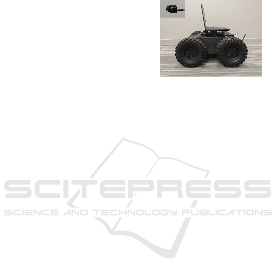
ing and testing phases. Initially, we calibrate our cam-

era, a FLIR Blackﬂy S, to estimate the intrinsics pa-

rameters of the camera (Fig. 1). The intrinsics pa-

rameters are utilized to build an accurate model of the

camera and simulate 3D points at varying distances

Figure 1: Dr. Robot Jaguar mobile robot platform with

FLIR Blackﬂy S camera onboard.

from the camera taken with inconstant mobile robot

velocities. These 3D points, using the camera model,

are projected onto the 2D plane. During the training

phase we observe the variability of the optical ﬂow

vector magnitudes and how these change with respect

to distance and velocity. The training phase which is

simulation-based is carried out ofﬂine. In addition,

using an accurate model of the camera we can sim-

ulate a very large number of 3D points that would

otherwise be impossible to observe using real-world

points and data. This entails a very descriptive proba-

bility distribution function that describes the relation-

ship between distance and velocity.

In our approach we employ the Lucas-Kanade op-

tical ﬂow algorithm (Lucas and Kanade, 1981) which

is a sparse optical ﬂow technique entailing in a faster

computation of motion vectors. In this research we

have used a single camera to implement optical ﬂow

and recognize places from the optical ﬂow patterns.

The camera is mounted on a mobile robot platform

(Fig. 1) along with a laptop computer with quad-core

Intel Core i7-8650U processor and 16GB of RAM.

No other sensors are utilized in this research. In addi-

tion, apart from the intrinsics of the camera no other

parameters are known. Camera velocity and distance

to 3D points are modeled during the training phase,

however, these two parameters are unknown during

testing phase.

3.1 Training Phase

During the training phase we observe the magnitude

variability of optical ﬂow vectors with respect to ve-

locity and distance. The mean and standard deviations

for velocity and distance are summarized in Table 1.

Both velocity and distance are drawn from Gaussian

probability distribution functions. The parameters

for velocity and distance used reﬂect the correspond-

ing parameters for velocity and depth in indoor and

outdoor environments where the mobile robot navi-

Modeling a priori Unknown Environments: Place Recognition with Optical Flow Fingerprints

795

gates with a relatively low velocity and the distance

to features is small in an indoor environment while

the velocity and distance are higher when navigating

through an outdoor environment .

Table 1: Modeling Parameters for Indoor and Outdoor En-

vironments.

Indoor Outdoor

Distance

(m)

µ = 1.5 µ = 20.0

σ = 0.4 σ = 5.0

Velocity

(km/m)

µ = 1.3 µ = 3.45

σ = 0.3 σ = 1.0

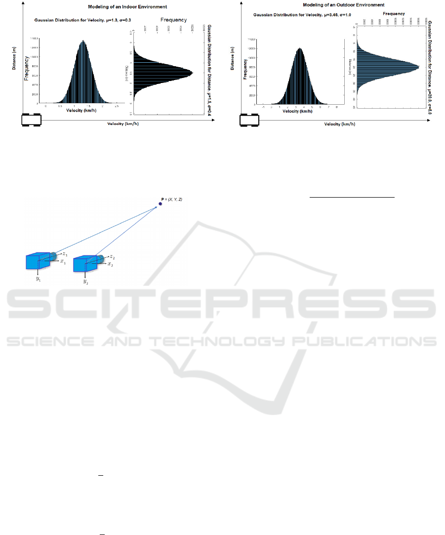
Figure 2 provides a pictorial representation of the

Gaussian distributions used for modeling camera ve-

locities and distances between camera and 3D points

(Fig. 3). We have observed 1 million, n = 10

, 3D

features with varying depths and velocities at which

they are observed. The overall simulation and pro-

jection of 3D points onto the 2D image plane of the

modeled camera required about 14.5 minutes (on a

quad-core Intel Core i7-8650U processor with 16GB

of RAM). For modeling the FLIR Blackﬂy S camera

we employed the (Corke, 2011) toolbox. Equation

1 shows the mathematical formulation for comput-

ing the mean magnitude, ||~u||, of all vectors given the

n = 10

3D points

~v =

∑

k=1

||~u

|| n = 1000000. (1)

The mean length, ~v, of the n optical ﬂow vectors

is then subtracted from each one of the n optical ﬂow

vectors as shown in (2)

= |~v −||~u

||| (2)

The resultant histogram derived by (2) is de-

scribed by a lognormal probability density function

(pdf) as expressed by (3)

= (δ;µ,σ) =

δσ

√

2π

−

(lnδ−µ)

2σ

δ > 0. (3)

The lognormal pdf acts as a likelihood estimator

for correlating the optical ﬂow patterns between the

training and testing phases. For inferring the prob-

abilistic score between the two patterns the cumula-

tive density function of the lognormal function is used

and, as expressed in (4)

(δ;µ,σ) =

er f c



−

lnδ −µ

√



= Φ



lnδ −µ



(4)

Further to this, following our methodology any

camera can be modeled and the optical ﬂow vectors

can be obtained by setting the parameters for veloc-

ity and distance. This approach greatly simpliﬁes the

modeling of an a priori unknown environment. Yet,

the parameters for velocity and distance can easily be

modiﬁed to model and simulate different types of en-

vironments on which the robot will navigate, for in-

stance, high-speed traversing of an outdoor environ-

ment. The modeled camera and its intrinsic matrix K

along with its corresponding values are shown in (5)





f /ρ

0 u

0 f /ρ

0 0 1









1682.4 0 757

0 1682.4 598

0 0 1





(5)

The resolution of the speciﬁc camera was set to

1440 ×1080 and the frame rate was approximately

12.3 frames/second. The focal length in mm was

estimated to be 5.80 mm, while the pixel size was

3.45 ×10

−6

µm and the diagonal ﬁeld of view (FOV)

' 58.42

◦

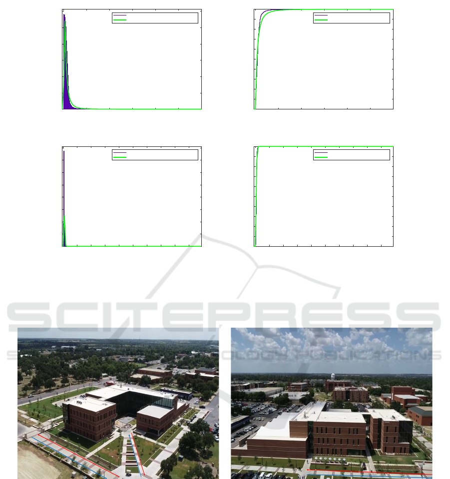
Figures 4 (a-b) depict the probability density func-

tion (PDF) and the cumulative density function (CDF)

of the lognormal function respectively, derived from

training using the parameters as shown in Table 1 for

an indoor environment. The estimated mean and stan-

dard deviation of the training PDF are µ = 1.93 and

σ = 1.17, respectively. In Figs. 4 (a) and (c) the his-

togram of the PDF depicts the variation of the length

of the optical ﬂow vectors with respect to distance and

velocity in a sample of 10

training repetitions. Fig-

ures 4 (c-d) depict the lognormal PDF and CDF for an

outdoor environment. The estimated mean and stan-

dard deviation of the training PDF are µ = 1.87 and

σ = 0.42.

3.2 Testing Phase

During the testing phase the robot navigates in a a pri-

ori unknown environment. The distance and velocity

of the navigating robot have to comply with the mod-

eled parameters of the training phase. Although this

is not a strict rule, observations from the testing en-

vironment have shown that the closer the real-world

parameters are to the modeled environment the better

and more accurate the similarity score will be. Dur-

ing testing, the robot takes continuous snapshots of

the environment and generates the optical ﬂow pat-

terns using the Lucas-Kanade optical ﬂow algorithm.

No images are stored nor is there a need for image

retrieval and comparison, only the properties of the

optical ﬂow vectors are stored in each pair of frames.

In particular, during testing the robot passes from

the same scene twice. At least two passes are neces-

sary for the robot to identify and recognize a scene.

VISAPP 2021 - 16th International Conference on Computer Vision Theory and Applications

796

(a) (b)

Figure 2: (a) Gaussian probability distribution functions used for modeling camera velocities and distances to features. The

mean and standard deviation for an indoor environment for velocity are µ = 1.3 and σ = 0.3 whereas mean distance and

standard deviation for distance are µ = 1.5 and σ = 0.4; (b) for an outdoor environment the velocity parameters are µ = 3.45

and σ = 1.0 whereas for distance are µ = 20.0 and σ = 5.0.

Figure 3: 3D point, P, observed by the same camera at two

different poses.

In the ﬁrst pass the robot captures images and gen-

erates the optical ﬂow patterns while in the second

pass the robot attempts to identify and recognize

whether a scene has previously been visited by the

robot by comparing the optical ﬂow patterns based on

the lognornal distributions generated during the train-

ing phase. The problem of place recognition is also

referred to as close looping where a robot tries to rec-

ognize a scene when the robot closes the loop (sec-

ond pass). In the ﬁrst pass we compute the midpoint

of each one of the vectors and then we compute the

midpoint of all midpoints, as shown in 6

¯x

, ¯y

∑

a=1

(6)

In the second pass, we again compute the mid-

point of all midpoints as described by 7

¯x

, ¯y

∑

b=1

(7)

Finally, we compute the Euclidean distances (eqn.

8) between the two optical ﬂow patterns (through their

midpoints) and we plug the result of it, δ, into our Cu-

mulative Distribution Function derived from the train-

ing data set which computes the similarity score be-

tween the ﬁrst pass and the second pass.

δ =

( ¯x

− ¯x

)

+ ( ¯y

− ¯y

)

(8)

The ﬁnal similarity score is computed using eqn.

P = 1 −P

(9)

3.3 Experiments

The following ﬁgures present the environments ex-

periments were carried out as well as the results ac-

complished. Figure 5 shows images of the outdoor

site used to carry out place recognition by traversing

three different routes depicted with red (ﬁrst pass) and

blue (second pass) vectors. (a) Routes 1 and 2 and (b)

route 3. Figure 6 shows images taken by the robot

from indoor and outdoor environments under varying

velocities and distances. In addition, the brightness of

images is not constant across all images. In the ﬁrst

column the reference images are shown while in the

rest of columns the images with the highest similar-

ity scores are depicted. In our results, there was only

one false positive which is shown in the third row of

the second column. The highest similarity scores for

two similar images is around 1% (1.76% for indoor

images) with a decreasing similarity score for images

which are less similar. For dissimilar images the sim-

ilarity score drops signiﬁcantly. As it can be seen the

similarity score is evidently high when the snapshots

are from the vicinity of the reference pose in spite of

the variation in velocities between the reference im-

age and the current robot snapshots.

Modeling a priori Unknown Environments: Place Recognition with Optical Flow Fingerprints

797

0 100 200 300 400 500

Data

0.01

0.02

0.03

0.04

0.05

0.06

Density

Histogram of vector magnitude variability

Lognormal fit (PDF)

0 100 200 300 400 500

Data

0.1

0.2

0.3

0.4

0.5

0.6

0.7

0.8

0.9

Cumulative probability

CDF of vector magnitude variability

Lognormal fit (CDF)

(a) (b)

0 100 200 300 400 500 600 700 800 900

Data

0.02

0.04

0.06

0.08

0.1

0.12

0.14

0.16

Density

Histogram of vector magnitude variability

Lognormal fit (PDF)

0 100 200 300 400 500 600 700 800 900

Data

0.1

0.2

0.3

0.4

0.5

0.6

0.7

0.8

0.9

Cumulative probability

CDF of vector magnitude variability

Lognormal fit (CDF)

Figure 4: (a-b) Indoor Environment: the histogram expresses the variability of the magnitude of the optical ﬂow vectors

with respect to distance and velocity. The ﬁtting functions are expressed with a lognormal Probability Distribution Function

(PDF) and a lognormal Cumulative Distribution Function (CDF). Mean and standard deviation are µ = 1.93 and σ = 1.17,

respectively; (c-d) Outdoor Environment: Mean and standard deviation are µ = 1.87 and σ = 0.42, respectively.

(a) (b)

Figure 5: Outdoor testing environment: Red vectors denote ﬁrst pass while blue vectors denote a second pass; (a) routes 1

and 2; (b) route 3.

4 CONCLUSIONS AND FUTURE

WORK

In this research we have implemented a method for

place recognition based on the similarity of optical

ﬂow ﬁngerprints. We have shown that using minimal

information about the environment as well as the sen-

sors employed it is feasible to model, train, and test

a robot to recognize places from the way an environ-

ment is perceived and not based on the characteristics

or the properties of the environment. In addition, we

have managed to exploit the advantages simulation

offers such as fast computations using large sample

data sets by providing the output of it to real-world

experiments.

VISAPP 2021 - 16th International Conference on Computer Vision Theory and Applications

798

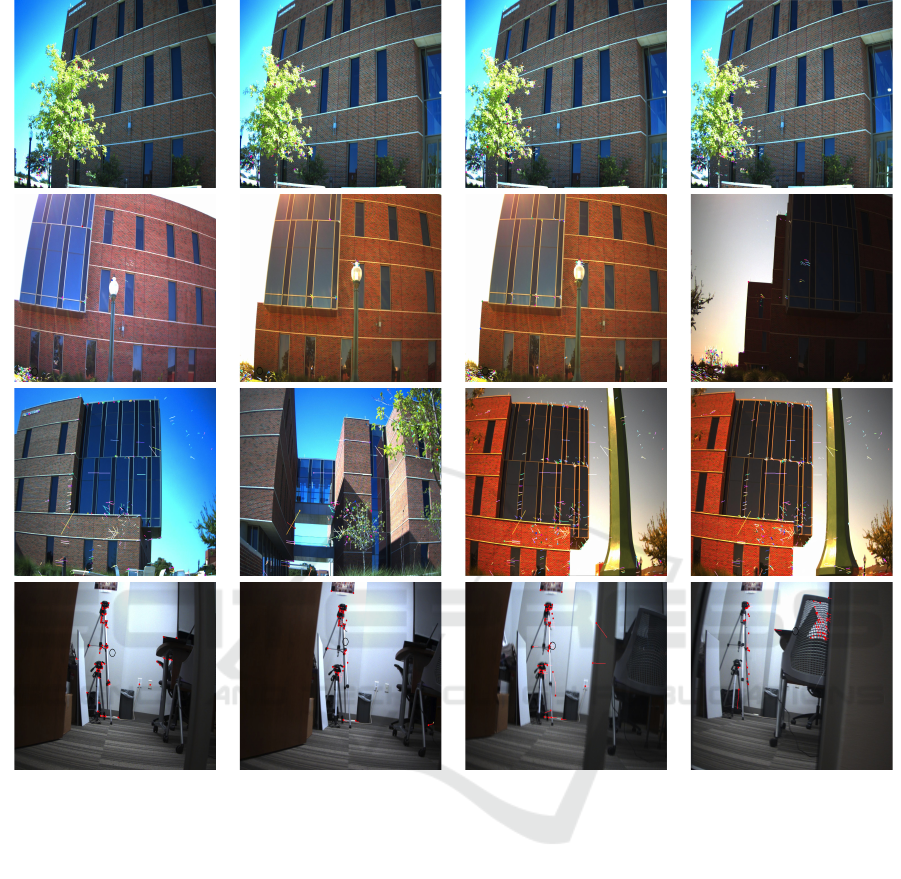
Figure 6: In the ﬁrst column the reference images are depicted while in columns 2-4 the images with the highest similarity

scores are depicted (from high to low). The ﬁrst three rows are from routes 1-3 while the last row is from an indoor ofﬁce

environment. In the second image of the third row it was the only false positive found. Images were captured with different

velocities and distances as well as varying illumination conditions.

As a future work we wish to extend this model

in several ways. First, we plan to incorporate into our

model methods that will allow the robot to navigate in

and recognize dynamic environments. A method we

will mostly be considering for dealing with dynamic

environments appears in (Cherubini and Chaumette,

2012). Second, we want implement the Kullback-

Leibler (KL) divergence for comparing different mul-

tivariate probability distribution functions that arise

from the optical ﬂow patterns. In that latter case,

training may not be necessary.

REFERENCES

Bardas, G., Astaras, S., Diamantas, S., and Pnevmatikakis,

A. (2017). 3D tracking and classiﬁcation system using

a monocular camera. Wireless Personal Communica-

tions, 92(1):63–85.

Barron, J. L., Fleet, D. J., and Beauchemin, S. S. (1994).

Performance of optical ﬂow techniques. International

Journal of Computer Vision, 12(1):43–77.

Bay, H., Ess, A., Tuytelaars, T., and Gool, L. V. (2008a).

Speeded-up robust features. Computer Vision and Im-

age Understanding, 110(3):346–359.

Bay, H., Ess, A., Tuytelaars, T., and Gool, L. V. (2008b).

Surf: Speeded up robust features. Computer Vision

and Image Understanding, 110(3):346–359.

Camus, T., Coombs, D., Herman, M., and Hong, T.-S.

Modeling a priori Unknown Environments: Place Recognition with Optical Flow Fingerprints

799

(1996). Real-time single-workstation obstacle avoid-

ance using only wide-ﬁeld ﬂow divergence. In Pro-

ceedings of the 13th International Conference on Pat-

tern Recognition, volume 3.

Cherubini, A. and Chaumette, F. (2012). Visual naviga-

tion of a mobile robot with laser-based collision avoid-

ance. The International Journal of Robotics Research,

32(2):189–205.

Corke, P. I. (2011). Robotics, Vision & Control: Fundamen-

tal Algorithms in Matlab. Springer.

Cummins, M. and Newman, P. (2008). Fab-map: Proba-

bilistic localization and mapping in the space of ap-

pearance. The International Journal of Robotics Re-

search, 27(6):647–665.

Diamantas, S. C. (2010). Biological and Metric Maps

Applied to Robot Homing. PhD thesis, School

of Electronics and Computer Science, University of

Southampton.

Diamantas, S. C., Oikonomidis, A., and Crowder, R. M.

(2010). Towards optical ﬂow-based robotic homing.

In Proceedings of the International Joint Conference

on Neural Networks (IEEE World Congress on Com-

putational Intelligence), pages 1–9, Barcelona, Spain.

Diamantas, S. C., Oikonomidis, A., and Crowder, R. M.

(2011). Biologically inspired robot navigation by ex-

ploiting optical ﬂow patterns. In Proceedings of the

International Conference on Computer Vision Theory

and Applications, pages 645–652, Algarve, Portugal.

Draper, S. O. B. A. (2011). Introduction to the bag of fea-

tures paradigm for image classiﬁcation and retrieval.

https://arxiv.org/abs/1101.3354, pages 1–25.

Gibson, J. J. (1974). The Perception of the Visual World.

Greenwood Publishing Group, Santa Barbara, CA,

USA.

Hrabar, S., Sukhatme, G., Corke, P., Usher, K., and Roberts,

J. (2005). Combined optic-ﬂow and stereo-based nav-

igation of urban canyons for a UAV. In Proceedings

of IEEE/RSJ International Conference on Intelligent

Robots and Systems, pages 302–309.

egou, H., Douze, M., Schmid, C., and P

erez, P. (2010).

Aggregating local descriptors into a compact image

representation. In 2010 IEEE Computer Society Con-

ference on Computer Vision and Pattern Recognition,

pages 3304–3311.

Kendoul, F., Fantoni, I., and Nonami, K. (2009). Optic ﬂow-

based vision system for autonomous 3d localization

and control of small aerial vehicles. Robotics and Au-

tonomous Systems, 57(6–7):591–602.

Liao, M., Shi, B., and Bai, X. (2018). Textboxes++: A

single-shot oriented scene text detector. IEEE Trans-

actions on Image Processing, 27(8):3676–3690.

Liao, M., Shi, B., Bai, X., Wang, X., and Liu, W. (2017).

Textboxes: A fast text detector with a single deep neu-

ral network. In AAAI.

Lowe, D. (1999). Object recognition from local scale-

invariant features. In Proceedings of the International

Conference on Computer Vision (ICCV ’99), pages

1150–1157, Corfu, Greece.

Lucas, B. D. and Kanade, T. (1981). An iterative image

registration technique with an application to stereo vi-

sion. In Proceedings of the 7th International Joint

Conference on Artiﬁcial Intelligence (IJCAI), August

24-28, pages 674–679.

Madjidi, H. and Negahdaripour, S. (2006). On robustness

and localization accuracy of optical ﬂow computation

for underwater color images. Computer Vision and

Image Understanding, 104(1):61–76.

Merrell, P. C., Lee, D.-J., and Beard, R. (2004). Obsta-

cle avoidance for unmanned air vehicles using opti-

cal ﬂow probability distributions. Sensing and Per-

ception, 5609:13–22.

Ohnishi, N. and Imiya, A. (2007). Corridor navigation and

obstacle avoidance using visual potential for mobile

robot. In Proceedings of the Fourth Canadian Confer-

ence on Computer and Robot Vision, pages 131–138.

Wang, H.-C., Finn, C., Paull, L., Kaess, M., Rosenholtz,

R., Teller, S., and Leonard, J. (2015). Bridging

text spotting and slam with junction features. In

2015 IEEE/RSJ International Conference on Intelli-

gent Robots and Systems (IROS), pages 3701–3708.

Warren, W. and Fajen, B. R. (2004). From optic ﬂow to

laws of control. In Vaina, L. M., Beardsley, S. A., and

Rushton, S. K., editors, Optic Flow and Beyond, pages

307–337. Kluwer Academic Publishers.

Zufferey, J.-C., Beyeler, A., and Floreano, D. (2008). Op-

tic ﬂow to control small uavs. In IEEE/RSJ Interna-

tional Conference on Intelligent Robots and Systems:

Workshop on Visual Guidance Systems for small au-

tonomous aerial vehicles, Nice, France.

VISAPP 2021 - 16th International Conference on Computer Vision Theory and Applications

800