EEG Classiﬁcation for Visual Brain Decoding via Metric Learning

Rahul Mishra and Arnav Bhavsar

Multimedia Analytics, Networks and Systems Lab, School of Computing & Electrical Engineering, IIT Mandi, India

Keywords:

CNN, Metric Learning, Siamese Network, Correlation Coefﬁcients, EEG Classiﬁcation, K-NN.

Abstract:

In this work, we propose CNN based approaches for EEG classiﬁcation which is acquired from a visual

perception task involving different classes of images. Our approaches involve deep learning architectures using

1D CNN (on time axis) followed by 1D CNN (on channel axis) and Siamese network (for metric learning)

which are novel in this domain. The proposed approaches outperform the state-of-the-art methods on the same

dataset. Finally, we also suggest a method to select fewer number of EEG channels.

1 INTRODUCTION

Brain decoding, in general, is not only an interest-

ing research area, but it also has beneﬁts from the

cognitive and clinical perspectives. In recent years,

there has been a considerable increment in the brain

decoding studies from EEG recordings. Typically, a

non-invasive brain-computer interface (BCI) based on

EEG is popularly used for decoding of mental emo-

tions/intentions (in a loose sense). A practical and

useful example of such decoding is, say, a BCI con-

trolled wheelchair or a BCI controlled user interface,

which can aid differently-abled people.

Since its discovery in 1924 by a German psychi-

atrist Hans Berger (Chen, 2014), electroencephalog-

raphy (EEG) was primarily used by health workers

for the applications like detection of seizure (Chen,

2014). However, over the years, its usage in the ﬁelds

of cognitive neuroscience and biomedical engineer-

ing has signiﬁcantly improved. The main beneﬁts of

this technique is not only its non-invasiveness but also

its high temporal resolution along with relatively low

cost, as compared to some other brain sensing de-

vices.

Apart from these advantages, EEG signals have

a disadvantage as very poor SNR. Having said that,

it is quite difﬁcult to assimilate what happens in the

brain of a person just from the EEG due to its poor

signal to noise ratio. Nevertheless, signiﬁcant amount

of successful works on BCI have been done for the

applications like decoding emotion and analyzing at-

tention (Chen et al., 2019; Craik et al., 2019; Gao

et al., 2015) etc.

Inspired by such research, we further explore a re-

cently considered direction of analyzing brain activity

generated while doing visual perception tasks (Tiru-

pattur et al., 2018). More speciﬁcally, in this work, we

propose a deep learning method to address the task of

EEG signal classiﬁcation to differentiate between the

perception of images (10 classes). The task involves

visual stimuli and imagination of images across dif-

ferent categories such as digits (0-9), characters (A-J),

and natural objects

Brain decoding from EEG signals can be car-

ried out with some traditional machine learning ap-

proaches for signal classiﬁcation (like KNN, SVM

etc.). These above methods are already well explored

in this area. However, for this study, we prefer to use

deep learning techniques, considering their superior

performance, in general, and in also different applica-

tion domains of EEG classiﬁcation.

A recent review and evaluation of deep learning

methods in solving different EEG-related tasks is re-

ported in (Craik et al., 2019), which discusses a vari-

ety of deep learning-based approaches. Such methods

also include the processing of EEG data to discrimi-

nate semantically distinct stimuli sources (Huth et al.,

2016). We observe via these works that it is useful to

thoughtfully consider combination of different neu-

ral networks modules to attempt to effectively address

and improve upon the state-of-the-art techniques in

EEG classiﬁcation tasks. Thus, in this work we con-

sider an in-house designed CNN model with 1D and

2D CNN modules, followed by a Siamese network,

which is motivated below.

As indicated earlier, in this work, we focus on

EEG data related to three different categories (Char-

acters, digits and objects). From an image perspective

160

Mishra, R. and Bhavsar, A.

EEG Classiﬁcation for Visual Brain Decoding via Metric Learning.

DOI: 10.5220/0010270501600167

In Proceedings of the 14th International Joint Conference on Biomedical Engineering Systems and Technologies (BIOSTEC 2021) - Volume 2: BIOIMAGING, pages 160-167

ISBN: 978-989-758-490-9

all these categories are well discriminative. Also, the

classes considered within each category are well dis-

criminative. However, it is not necessary that the dis-

criminability of features at the image domain (which

leads to very high image classiﬁcation performance),

also reﬂects in discrimination of the corresponding

EEG signals.

One way to improve the discrimination in the EEG

domain is to take the advantage of metric learning

(Kaya and Bilge, 2019). Metric learning is a method

which is based on a distance metric that aims to learn

the similarity or dissimilarity between samples. The

objective of metric learning is learn a feature space

which helps in not only reducing the distance between

similar objects, but, also in increasing the distance be-

tween dissimilar objects. A common network which

is for metric learning is the Siamese network (Brom-

ley et al., 1994). Thus, in addition to an in-house but

a more traditional CNN network, we also employ a

Siamese network in this work, which, as yet has not

been considered in many EEG related tasks.

2 RELATED WORK

Signiﬁcant amount of literature is available on EEG

analysis for different applications, that used tradi-

tional machine learning approaches. However, in line

with the methods used in this paper, we only discuss

works that have employed the contemporary deep

learning methods.

A large fraction of works based on EEG classiﬁ-

cation using deep learning mainly focus on tasks like

seizure detection (Chen, 2014; Oweis and Abdulhay,

2011),event-related potential detection (Parekh et al.,

2017), emotion recognition (Chen et al., 2019), men-

tal workload (Di Flumeri et al., 2018), motor imagery

(He et al., 2018) and sleep scoring (Ghimatgar et al.,

2019) etc. The authors in (Craik et al., 2019) dis-

cussed the signiﬁcant practices and outcomes based

on deep learning for the task of EEG classiﬁcation.

In (Gao et al., 2015; Chen et al., 2019), the au-

thors propose the use of well known deep learning

techniques (KNN, fully connected ANN and CNN)

to learn the features and to use these features for the

classiﬁcation of emotions with EEG signals. Another

attempt to the classiﬁcation of emotions using EEG

signals was successfully done in (Chen et al., 2019).

Here, the authors proposed a deep convolution neural

network (CNN) based on the combination of temporal

and frequential features. They worked with the DEAP

dataset for EEG-based emotion classiﬁcation (Koel-

stra et al., 2011). The authors of (Schirrmeister et al.,

2017; Bashivan et al., 2015) tried with the combina-

tion of CNN and LSTM architectures to classify EEG

signals for different tasks.

Some of the current research involve identifying

patterns from EEG to recognize the stimuli that give

rise to speciﬁc responses (Spampinato et al., 2016;

Huth et al., 2016). The work in (Parekh et al., 2017)

is also a recent work wherein the authors suggested

an image annotation system that works with EEG sig-

nals.This study comes with the usage of P300 ERP

signature for purpose of image annotation. We can

understand P300 as an event-related potential (ERP)

component which is obtained in the process of taking

a decision about an event (Linden, 2005).

Some of the recent research also includes the

investigation of visualizing brain activity of a sub-

ject performing visual task (Nishimoto et al., 2011).

Apart from EEG signals, fMRI can also be used to de-

code human brain. One attempt for this type of work

has been done by (Nishimoto et al., 2011). They

have used fMRI images to envision the stimuli in the

EEG signal while watching a short movie clip. The

advantage of brain activity captured through fMRI is

its high spatial resolution, but, it is not cost effective.

This drawback can be overcome by lower cost tech-

niques (such as EEG). EEG provide a higher tem-

poral resolution compared to fMRI. A large number

of cognitive studies have showed that multiple object

categories can be interpreted in event related poten-

tial (ERP) with EEG (Carlson et al., 2011; Simanova

et al., 2010; Wang et al., 2012).

However, limited number of techniques have been

suggested (Kapoor et al., 2008) to address the prob-

lem of decoding the EEG signals associated with the

task of visual perception and majority of these tech-

niques were devised for binary classiﬁcation (e.g.,

presence or absence of a given object class).

One of a very recent approach that deals with the

EEG classiﬁcation for the task of visual perception is

given by (Tirupattur et al., 2018). In this work the au-

thors proposed a deep learning network for the clas-

siﬁcation of EEG signals while the signals has been

captured by Emotiv Epoc (14- channels) device (Styt-

senko et al., 2011). Parallel to this work, the authors

of (Jolly et al., 2019) also proposed a GRU based

deep learning approach to classify the EEG signals

from the ThoughtViz dataset (Tirupattur et al., 2018).

But, still there are very limited methods available for

brain decoding studies. We consider these works as

novel early baseline methods, for our work as we no-

tice scope of improvement in this domain.

Considering the above, the main contribution of

this paper can be listed as follows:

1. This paper is an attempt to develop an improved

visual stimuli evoked EEG classiﬁer having em-

EEG Classiﬁcation for Visual Brain Decoding via Metric Learning

161

phasis on following techniques:

(a) An in-house designed CNN architecture.

(b) Distance-metric based learning via a Siamese

network which involves the above network ar-

chitechture as its component.

2. We also consider the fact that not all channels

may be equally important for classiﬁcation, and

present a correlation based technique to select

fewer number of relevant EEG channels.

All the works presented here are based on a publicly

available dataset (details are in subsequent sections).

3 DATASET DETAILS

The dataset for this work is a publicly available

dataset which is acquired from Tirupattur et al.’s work

(Tirupattur et al., 2018). Before this work (Tiru-

pattur et al., 2018) this dataset was originally re-

leased by Kumar et al.’s (Kumar et al., 2018). Orig-

inally, this contains EEG recordings of 23 volunteers

who were shown stimuli of three different categories

(characters(A-J), digits(0-9) and objects(10 classes

from ImageNet dataset)).

From each category 10 examples are chosen.

Figure 1: Samples from MNIST, ImageNet &

char74k (Deng, 2012; Deng et al., 2009; de Campos

et al., 2009).

Each of these examples have EEG signals from 23

volunteers for all 10 classes of images and each EEG

recording is of 10 seconds. This EEG data is collected

using Emotiv Epoc headset.The electrodes location

for Emotiv Epoc is given in ﬁgure 2 (Mehmood and

Lee, 2016). This device contains 14 channels and the

sampling frequency is 128 Hz.

The authors of (Tirupattur et al., 2018) created

smaller chunks of EEG data by using a sliding win-

dow of 32 samples with overlapping of 8 samples.

Figure 2: Electrodes location for Emotiv Epoc.

No pre-processing or transformation of the data has

been done in our approach and the data is used as

in the form released by Tirupattur et al. (Tirupattur

et al., 2018). We carried out experiments with the

proposed method on all the three types of data. The

results of ThoughtViz (Tirupattur et al., 2018) are pri-

marily taken as a baseline for this work, along with a

couple of other methods which have reported results

on some selected classiﬁcation tasks. These are used

for comparison in section 5.

4 METHODOLOGY

In this section we discuss the two classiﬁcation mod-

els and the channel selection approach in the follow-

ing subsections.

4.1 EEG Classiﬁcation

As EEG signals have very low signal to noise ratio,

it is important to extract / learn relevant features for

the classiﬁcation task. One effective way to execute

this task is the use of convolution neural networks,

which inherently involves the neighbourhood context

of each sample from each channel across time. Fur-

ther, for increasing robustness one can also consider

the convolution across channel axis. This intuition

motivates us to employ a 1D CNN across time fol-

lowed by 1D CNN across channels which enables

us to consider the neighbouring context information

of both directions. Below we describe the two ap-

proaches proposed in this work. The ﬁrst one is a

base in-house network consisting of 1D convolutions,

and the second one is a Siamese network, built upon

the base network.

4.1.1 Base CNN Network

The details of base deep learning model is given be-

low:

The input data is of the dimension (14 x 32) (i.e. 14

channels and 32 samples)

1. Apply 1D CNN on each individual channel to cap-

ture context information across time axis.

2. Apply 1D CNN on channel axis to capture neigh-

bourhood context across channels.

3. Maxpool layer is further applied, which is known

to yeild some robustness against intra-class varia-

tion.

4. After maxpool layer, we again apply a 1D CNN

on time axis of the signal.

BIOIMAGING 2021 - 8th International Conference on Bioimaging

162

5. Finally, the features extracted from the ﬁnal CNN

layer, are input to a classiﬁer layer made up of

dense layers, followed by a softmax output layer.

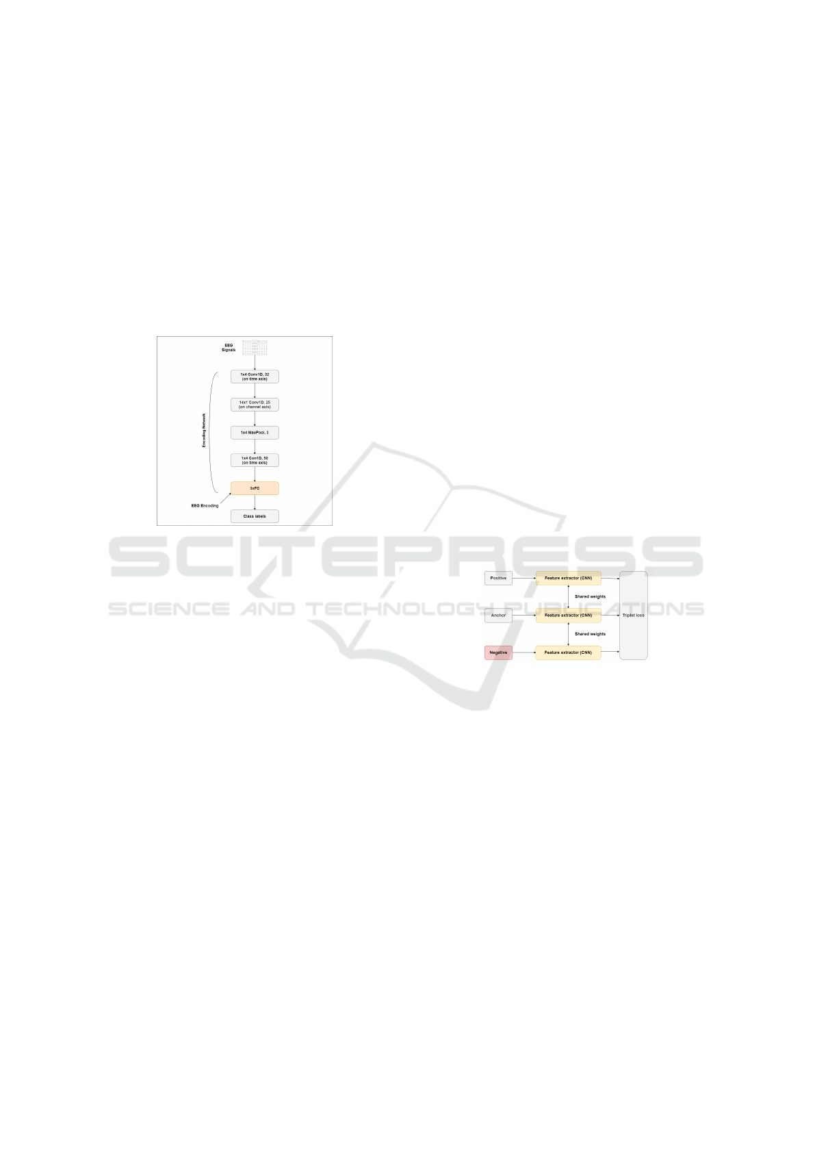
The architecture is depicted in Figure 3. The num-

bers in each block, denote the number of convolution

ﬁlters for that block. The fully connected layers con-

tain 500, 128 and 32 neurons. The ﬁnal softmax layer

is of the size equal to the number of classes. ReLU

activation has been used after each of the internal lay-

ers. We train the classiﬁers with adam optimizer, with

a batch size of 64 and learning rate of 1e-4. We train

this network from scratch.

Figure 3: Network architecture for EEG classiﬁcation.

4.1.2 Siamese Network

As indicated earlier, a Siamese network is a useful

approach to learn features based on the similarity and

dissimilarity of input data, so that, ideally the learnt

embeddings, are similar for the data of the same class

and dissimilar otherwise. We believe that such a

transformation is particularly useful to be considered

for EEG classiﬁcation, which involves noisy data. It

helps to improve separability in between classes.

A popular variant of the Siamese network works

on the minimization of triplet loss (Dong and Shen,

2018). Triplet loss is a recent and popular loss func-

tion for machine as well as deep learning algorithms.

The main idea of this loss function is the comparison

of a baseline (anchor) input to a positive (true) input

and a negative (false) input. The main motive behind

this comparison is to minimize the distance between

baseline (anchor) input and positive (true) input and

to maximize the distance between baseline (anchor)

input to the negative (false) input.

Mathematically, we can write the distance for a pair

of input samples (X

, X

) as,

, X

) =k G

) − G

) k (1)

Here, G

) and G

) are the transformation of

input data. This transformation embeds the data into

a new space which satisﬁes the purpose of distance-

metric learning.

Siamese network works on the creation of triplets

and further task is the minimization of triplet loss.

Triplet loss for Siamese network can be given by

equation

a =k (G

(X)− G

)) k

(2)

b =k (G

(X)− G

)) k

(3)

Triplet

= max(0, a − b + α) (4)

Here,

X = input anchor vector

= input negative vector

= input positive vector

α = margin between positive and negative pairs

The selection of triplets for training the Siamese net-

work is an important aspect (Chang et al., 2019). Typ-

ically, there are two ways to select triplets.

a) Manually or ofﬂine: In this approach, we ﬁrst gen-

erate the triplets manually (often randomly) and then

ﬁt the data to the base network.

b) Online: In this approach, we feed a batch of train-

ing data, generate triplets using all examples in the

batch and calculate the loss on it. While the batch

is selected randomly, those triplets are selected which

yield a smaller loss.

Figure 4: Siamese architecture.

The overall architecture of the Siamese network

is shown in Fig 4, where each of the CNN model

is essentially some base network, with the same ar-

chitecture. All the three CNN models are trained si-

multaneously (hence, the weights are shared) and we

can choose any one of them for testing after complete

training. In our case, after complete training of the

base network (in the previous subsection), we use this

network as a base network for Siamese. We removed

the last layer (softmax layer) of the base network and

enable the training of all the parameters. We use both

the above methods of triplet selection for our experi-

ments.

4.2 Channel Selection

Channel selection is about selecting fewer channels

instead of all available channels. The importance of

channel selection can be illustrated from these points:

EEG Classiﬁcation for Visual Brain Decoding via Metric Learning

163

1. Extracting features only from the relevant chan-

nels can reduce the computational complexity

while performing any EEG signal processing.

2. The use of unnecessary channels might results

into the overﬁtting, which can degrade the perfor-

mance the overall system.

We present a correlation-based technique for channel

selection. Essentially, we can remove a channel from

being considered if the correlation of that channel is

high with respect to some other channel. A correla-

tion coefﬁcient is a measure of statistical relationship

in between two variables. The variation in the value

of correlation coefﬁcient can only be in between -1

to +1. If the value of the correlation coefﬁcient is

high, that means the variables are highly related to

each other. The correlation coefﬁcient can be found

with this equation.

R =

∑

xy) − (

∑

x)(

∑

[N(

∑

) − (

∑

][N(

∑

) − (

∑

]

(5)

Here,

R = correlation coeff.

x, y = input samples

N = total number of samples

Correlation matrix of each dataset can be calculated

by taking average of correlation matrix of all the sam-

ples. This gives the average relationship of each chan-

nel with other channels for that dataset. Since, this is

an initial work, we have used simplistic channel se-

lection approach. However, one may consider other

feature selection methods.

5 EXPERIMENTS

Below we provide the results of our experiments with

the ThoughtViz dataset and our deep network models.

We use the same splitting for training and test data as

released by (Tirupattur et al., 2018). The ratio of

training and test data is roughly (90:10). The number

of training and test samples for Character dataset are

45083 and 5642 respectively. The number of train-

ing and test samples for MNIST dataset are 44367

and 5642 respectively. The number of training and

test samples for object dataset are 45390 and 5706 re-

spectively.

5.1 Results

Below we provide the results for the coarse level clas-

siﬁcation (between 3 broad categories), followed by

ﬁne level classiﬁcation (within each category of digit,

character, and objects).

5.1.1 Coarse Level EEG Classiﬁcation

We ﬁrst report our experiment involving classiﬁcation

between the three broad categories of the datasets (i.e.

characters, digits and object). Thus, this is a 3-class

classiﬁcation task. We use the network as discussed

in section 4.1.1 and with softmax activation at the out-

put. We train this network from scratch. The coarse

level classiﬁcation task had only been performed by

(Kumar et al., 2018),and not by any other research

group. So we are comparing our results with this only.

The detailed results are given in Table 1. The re-

sults are showing signiﬁcant improvement over the

work in (Kumar et al., 2018).

Table 1: Coarse level classiﬁcation acc. (overall).

Dataset Accuracy Accuracy

for the for

proposed (Kumar et al., 2018)

network

ThoughtViz 89.5% 85.2%

The detailed category wise results are given in Table

2. It can be noted that for all three classes, the classi-

ﬁcation accuracy is consistently high.

Table 2: Coarse level classiﬁcation acc. (individual).

Category True predict Total samples Acc.

Character 5032 5642 89.18%

Digits 5050 5642 89.5%

Object 5132 5706 89.9%

5.1.2 Fine Level EEG Classiﬁcation

The result and the improvement for the coarse classi-

ﬁcation is quite encouraging and motivates us to per-

form the ﬁne level classiﬁcation of the image classes

within each of individual broad categories.

Since each dataset (character, digits and objects)

contains 10 classes, hence, it is a 10 class classiﬁ-

cation problem for each dataset. For the comparison

purpose, we are taking the results of Tirupattur et al.’s

work (Tirupattur et al., 2018).

We ﬁrst provide the results using the architecture

explained in Section 4.1.1. We trained three differ-

ent softmax classiﬁers with this architecture (since we

have three EEG datasets).All three models are trained

from scratch.

For the implementation of Siamese network, we

take the trained network as used in section 4.1.1 as our

feature extractor (without the fully connected classi-

ﬁcation layer). The triplet loss has been used as the

loss function for this network. After minimization of

loss, we used k-nearest neighbour as a classiﬁer for

this network. As a start of the classiﬁcation task with

Siamese network we manually created triplets and an-

alyze classiﬁcation accuracy of this model.

BIOIMAGING 2021 - 8th International Conference on Bioimaging

164

Although the performance is still better than the

comparative method of (Tirupattur et al., 2018), they

do not show improvement over our earlier results of

the single CNN network of Section 4.1.1.

From these results, we conclude that the selected

triplets in the above strategy may not be good enough

to train the Siamese network properly. So, in order

to prepare better triplets and proper minimization of

triplet loss we use a different strategy for the training

of Siamese networks i.e. Online training. The details

of this training are given in Section 4.1.2. All results

from the above experiments are given in Table 3.

Table 3: Classiﬁcation accuracy from different methods.

Methods Datasets

Object Digits Characters

(Tirupattur et al., 2018) 72.95% 72.88% 71.18%

(Jolly et al., 2019) 77.4% NA NA

Proposed base model 76.253% 75.647% 74.264%

Siamese model (ofﬂine) 75.9% 75.2% 73.8%

Siamese model (online) 77.9 % 76.2% 74.8%

From the results in Table 3, we clearly observe the

improvement using the Siamese network over not just

the previous methods but also our earlier results. Note

that the authors of (Jolly et al., 2019) only performed

their classiﬁcation task with object dataset. Thus, this

indicates that while the Siamese network can indeed

learn a more discriminative feature space, it is impor-

tant to select the triplet using an appropriate method.

5.2 Channel Selection

After getting motivating results for both coarse level

as well ﬁne level EEG classiﬁcation, we now report

the results with the channel selection process. The

need for channel selection is already discussed in sec-

tion 4.2.

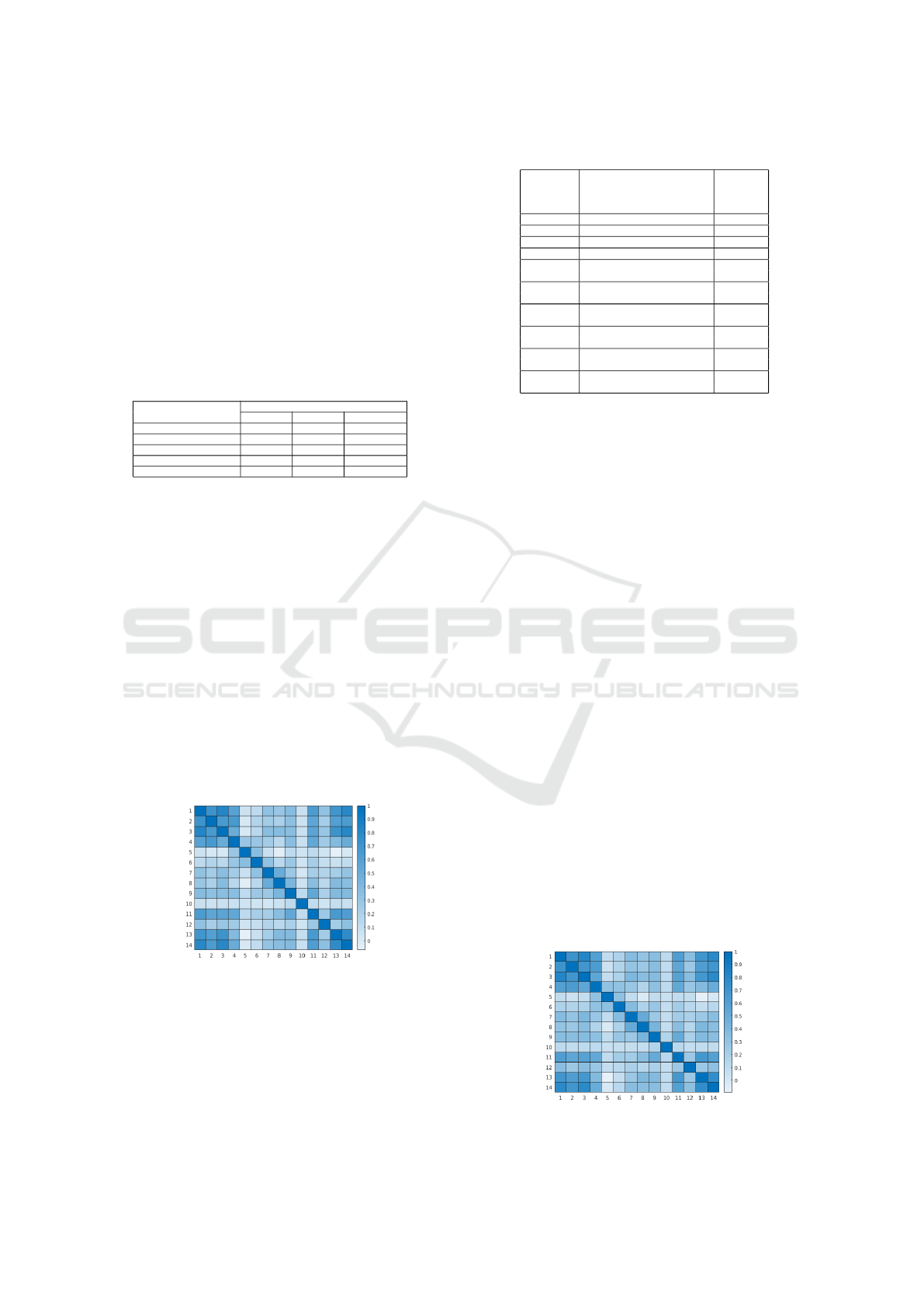
Figure 5: Correlation matrix for Object dataset.

We applied correlation based technique for the

search of relevant channels. Calculating the corre-

lation coefﬁcient is a statistical way to ﬁnd the sim-

ilarity measure between two variables (details given

in section 4.2). With the estimation of correlation co-

efﬁcient, we can ﬁgure out the most similar channel

pairs and can choose one of them instead of both. By,

Table 4: Channel selection with correlation(Object).

Threshold Channels Removed Classi.

with less

channels

C ≥ 0.8 F3 & AF4 75.7%

C≥ 0.7 F3, AF4 & F8 74%

C≥ 0.6 AF3 , F3, AF4 & F8 73.85%

C ≥ 0.5 F7, AF3 ,FC6, F3, AF4 & F8 73.659%

C ≥ 0.4 AF3, F7, F3, O2 , FC6, F8 73.5%

, AF4

C ≥ 0.3 AF3, F7, F3, FC5 , O2 , FC6 70.9%

, F8, AF4

C ≥ 0.2 AF3, F7, F3, FC5 , P7, O2 68.2%

, P8,FC6, F8, AF4

C≥ 0.1 AF3, F7, F3, FC5 , P7, O2 67.3%

, P8, FC6, F4, F8, AF4

C≥ 0.05 AF3, F7, F3, FC5, T7, P7 67%

, O2, P8, FC6, F4, F8, AF4

C≥ 0.01 AF3, F7, F3, FC5, T7, P7 66.3%

, O2, P8, T8, FC6, F4, F8, AF4

this way we can choose fewer number of the more

distinctly informative channels. This method can be

executed with the estimation of individual correlation

matrices for the individual dataset (i.e object, digits

and characters). The overall correlation matrix for a

dataset is the average of all correlation matrices for all

training samples from that dataset.

The correlation matrix of each individual dataset

is given below in ﬁgure 5, 6 and 8. Each entry of

this correlation matrix indicates the similarity of one

channel with respect to the other channel.

In order to remove the channels, we choose a pair

which has a high correlation coefﬁcient. To properly

assess this process we consider the similarity with dif-

ferent thresholds on the correlation values (from 0.8

to 0.1 in steps of 0.1). If the correlation coefﬁcient

of a pair is greater than that threshold, we select only

one entry from that pair. The detailed results with this

analysis are given in Tables 4, 5 and 6. For simplic-

ity, the classiﬁcation in case of the channel selection

was performed using the base CNN model described

in Section 4.1.1. For, estimating the classiﬁcation ac-

curacy we take the remaining channels after removal

of the redundant channels. Graphically, we can show

the variation of classiﬁcation accuracy with channels

in the given ﬁgure 7. Here, y-axis represents the clas-

siﬁcation accuracy (%) while the x-axis represents the

number of channels. From all of these tables and ﬁg-

ure, we can conclude that the classiﬁcation accuracy

Figure 6: Correlation matrix for Char74K dataset.

EEG Classiﬁcation for Visual Brain Decoding via Metric Learning

165

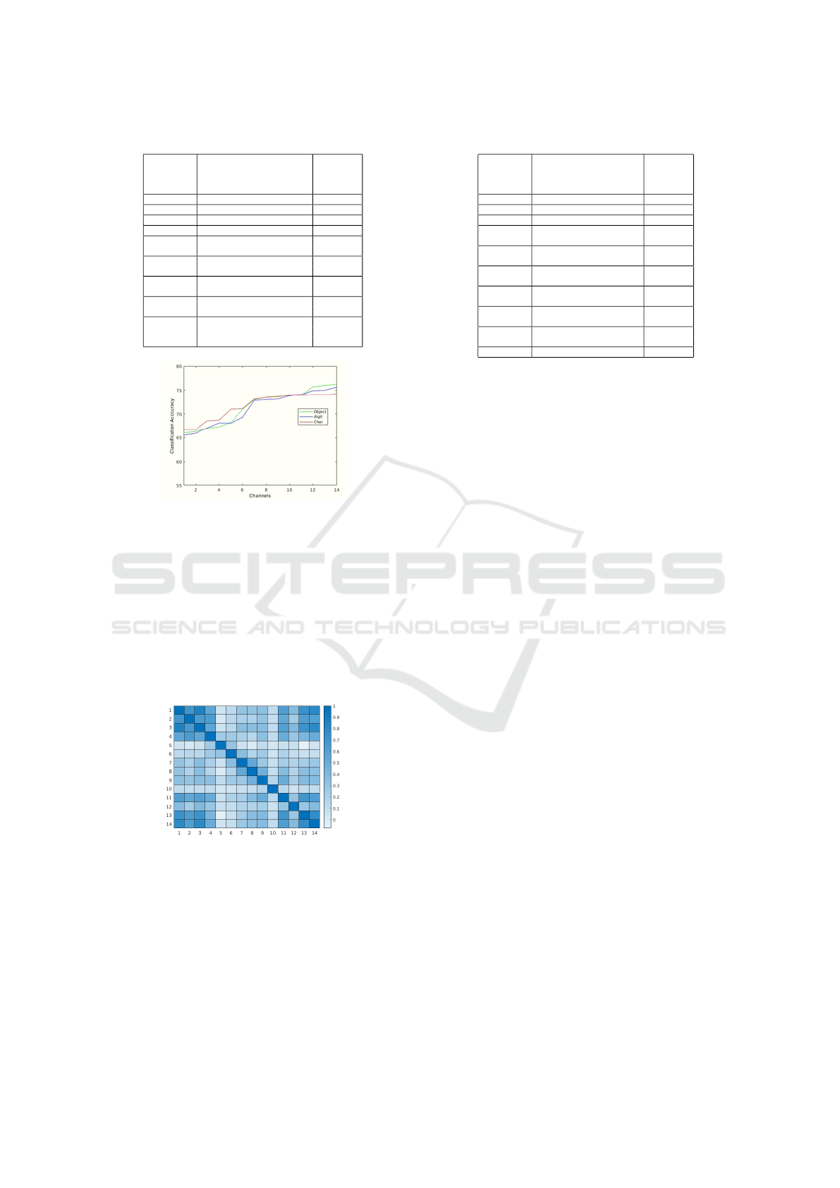
Table 5: Channel selection with correlation (Char dataset).

Threshold Channels Removed Classi.

Acc.

with less

channels

C ≥ 0.8 AF3 74.02%

C≥ 0.7 AF3, AF4 73.9%

C≥ 0.6 AF3 , F7, F8 & AF4 73.9%

C ≥ 0.5 AF3 ,F7, F3, FC6, F8 & AF4 73.6%

C ≥ 0.4 AF3 ,F7, F3, O2 , FC6, F8 73.46%

& AF4

C ≥ 0.3 AF3 ,F7, F3, FC5 ,P7, O2 71.1%

, FC6, F8 & AF4

C ≥ 0.2 AF3 ,F7, F3, FC5 ,P7, O1 68.7%

, O2 ,FC6, F8 & AF4

C≥ 0.1 AF3 ,F7, F3, FC5 ,P7, O1 68.557%

, O2, P8, ,FC6, F8 & AF4

C≥ 0.05 AF3 ,F7, F3, FC5 ,T7 , P7, 66.67%

O1, O2, P8, FC6, F4, F8

& AF4

Figure 7: Variation of classiﬁcation accuracy with channels

(Object dataset).

is highest when all channels taken into account i.e

each channel can be said to contribute for the clas-

siﬁcation. However, even if we remove few channels

the classiﬁcation accuracy in not dropping drastically.

This observation is valid for all the 3 classiﬁcation

tasks. Hence, for those application where the com-

putational and memory necessities increase with the

increase in the number of channels, we can work with

limited number of relevant channels.

Figure 8: Correlation matrix for MNIST dataset.

6 DISCUSSION & CONCLUSION

In this work, we have proposed approaches for EEG

signal classiﬁcation for the task involving visual stim-

uli, involving different categories of images. The ex-

periments with the different model architectures lead

us to the ﬁnal model which is giving a signiﬁcant im-

provement in the classiﬁcation accuracy with respect

Table 6: Channel selection with correlation (MNIST).

Threshold Channels Removed Classi.

Acc.

with less

channels

C ≥ 0.8 AF3, 74.9%

C≥ 0.7 AF3, F8, AF4 74.08%

C≥ 0.6 AF3, F7, F3, F8, AF4 73.8%

C ≥ 0.5 AF3, F7, F3, O1, FC6, F8 73.1%

, AF4

C ≥ 0.4 AF3, F7, F3, O1, O2, FC6 72.84%

, F8, AF4

C ≥ 0.3 AF3, F7, F3, FC5, P7, O1 69.248%

, O2, FC6,F8, AF4

C ≥ 0.2 AF3, F7, F3, FC5, P7 68.1%

, O1, O2, P8, FC6 , F8, AF4

C≥ 0.1 AF3, F7, F3, FC5, P7, O1 68.1%

, O2, P8, FC6 , F8, AF4

C≥ 0.05 AF3, F7, F3, FC5 ,T7, P7 67.06%

, O1, O2, P8, FC6, F8, AF4

C≥ 0.01 removed all except F4 65.9%

to the all available state of the art methods. After get-

ting the suitable EEG classiﬁer we further improve

the classiﬁcation results using the concept of distance-

metric learning via a Siamese network with a triplet

loss and using online triplet selection. Finally, we also

suggest using less number of channels and demon-

strate the effectiveness of a correlation based channel

selection strategy to reduce the number of channels,

without signiﬁcantly reducing the classiﬁcation accu-

racy. While we have improved the state-of-the-art per-

formance, we still believe that there is further scope of

improvement and analysis.

REFERENCES

Bashivan, P., Rish, I., Yeasin, M., and Codella, N.

(2015). Learning representations from eeg with

deep recurrent-convolutional neural networks. arXiv

preprint arXiv:1511.06448.

Bromley, J., Guyon, I., LeCun, Y., S

ackinger, E., and Shah,

R. (1994). Signature veriﬁcation using a” siamese”

time delay neural network. In Advances in neural in-

formation processing systems, pages 737–744.

Carlson, T. A., Hogendoorn, H., Kanai, R., Mesik, J., and

Turret, J. (2011). High temporal resolution decod-

ing of object position and category. Journal of vision,

11(10):9–9.

Chang, S., Li, W., Zhang, Y., and Feng, Z. (2019). Online

siamese network for visual object tracking. Sensors,

19(8):1858.

Chen, G. (2014). Automatic eeg seizure detection using

dual-tree complex wavelet-fourier features. Expert

Systems with Applications, 41(5):2391–2394.

Chen, J., Zhang, P., Mao, Z., Huang, Y., Jiang, D., and

Zhang, Y. (2019). Accurate eeg-based emotion recog-

nition on combined features using deep convolutional

neural networks. IEEE Access, 7:44317–44328.

Craik, A., He, Y., and Contreras-Vidal, J. L. (2019). Deep

learning for electroencephalogram (eeg) classiﬁca-

tion tasks: a review. Journal of neural engineering,

16(3):031001.

BIOIMAGING 2021 - 8th International Conference on Bioimaging

166

de Campos, T. E., Babu, B. R., and Varma, M. (2009). Char-

acter recognition in natural images. In Proceedings

of the International Conference on Computer Vision

Theory and Applications, Lisbon, Portugal.

Deng, J., Dong, W., Socher, R., Li, L.-J., Li, K., and Fei-

Fei, L. (2009). Imagenet: A large-scale hierarchical

image database. In 2009 IEEE conference on com-

puter vision and pattern recognition, pages 248–255.

Ieee.

Deng, L. (2012). The mnist database of handwritten digit

images for machine learning research [best of the

web]. IEEE Signal Processing Magazine, 29(6):141–

142.

Di Flumeri, G., Borghini, G., Aric

o, P., Sciaraffa, N., Lanzi,

P., Pozzi, S., Vignali, V., Lantieri, C., Bichicchi, A.,

Simone, A., et al. (2018). EEG-based mental work-

load neurometric to evaluate the impact of different

trafﬁc and road conditions in real driving settings.

Frontiers in human neuroscience, 12:509.

Dong, X. and Shen, J. (2018). Triplet loss in siamese net-

work for object tracking. In Proceedings of the Euro-

pean Conference on Computer Vision (ECCV), pages

459–474.

Gao, Y., Lee, H. J., and Mehmood, R. M. (2015). Deep

learninig of eeg signals for emotion recognition. In

2015 IEEE International Conference on Multimedia

& Expo Workshops (ICMEW), pages 1–5. IEEE.

Ghimatgar, H., Kazemi, K., Helfroush, M. S., and Aarabi,

A. (2019). An automatic single-channel eeg-based

sleep stage scoring method based on hidden markov

model. Journal of neuroscience methods, page

108320.

He, Y., Eguren, D., Azor

ın, J. M., Grossman, R. G., Luu,

T. P., and Contreras-Vidal, J. L. (2018). Brain–

machine interfaces for controlling lower-limb pow-

ered robotic systems. Journal of neural engineering,

15(2):021004.

Huth, A. G., Lee, T., Nishimoto, S., Bilenko, N. Y., Vu,

A. T., and Gallant, J. L. (2016). Decoding the seman-

tic content of natural movies from human brain activ-

ity. Frontiers in Systems Neuroscience, 10:81.

Jolly, B. L. K., Aggrawal, P., Nath, S. S., Gupta, V., Grover,

M. S., and Shah, R. R. (2019). Universal eeg en-

coder for learning diverse intelligent tasks. In 2019

IEEE Fifth International Conference on Multimedia

Big Data (BigMM), pages 213–218. IEEE.

Kapoor, A., Shenoy, P., and Tan, D. (2008). Combining

brain computer interfaces with vision for object cat-

egorization. In 2008 IEEE Conference on Computer

Vision and Pattern Recognition, pages 1–8. IEEE.

Kaya, M. and Bilge, H. S¸. (2019). Deep metric learning: A

survey. Symmetry, 11(9):1066.

Koelstra, S., Muhl, C., Soleymani, M., Lee, J.-S., Yazdani,

A., Ebrahimi, T., Pun, T., Nijholt, A., and Patras, I.

(2011). Deap: A database for emotion analysis; using

physiological signals. IEEE transactions on affective

computing, 3(1):18–31.

Kumar, P., Saini, R., Roy, P. P., Sahu, P. K., and Dogra, D. P.

(2018). Envisioned speech recognition using eeg sen-

sors. Personal and Ubiquitous Computing, 22(1):185–

199.

Linden, D. E. (2005). The p300: where in the brain is it

produced and what does it tell us? The Neuroscientist,

11(6):563–576.

Mehmood, R. M. and Lee, H. J. (2016). Towards human

brain signal preprocessing and artifact rejection meth-

ods. In Int’l Conf. Biomedical Engineering and Sci-

ences, pages 26–31.

Nishimoto, S., Vu, A. T., Naselaris, T., Benjamini, Y., Yu,

B., and Gallant, J. L. (2011). Reconstructing vi-

sual experiences from brain activity evoked by natural

movies. Current Biology, 21(19):1641–1646.

Oweis, R. J. and Abdulhay, E. W. (2011). Seizure classiﬁ-

cation in eeg signals utilizing hilbert-huang transform.

Biomedical engineering online, 10(1):38.

Parekh, V., Subramanian, R., Roy, D., and Jawahar, C.

(2017). An eeg-based image annotation system. In

National Conference on Computer Vision, Pattern

Recognition, Image Processing, and Graphics, pages

303–313. Springer.

Schirrmeister, R. T., Springenberg, J. T., Fiederer, L. D. J.,

Glasstetter, M., Eggensperger, K., Tangermann, M.,

Hutter, F., Burgard, W., and Ball, T. (2017). Deep

learning with convolutional neural networks for eeg

decoding and visualization. Human brain mapping,

38(11):5391–5420.

Simanova, I., Van Gerven, M., Oostenveld, R., and Hagoort,

P. (2010). Identifying object categories from event-

related eeg: toward decoding of conceptual represen-

tations. PloS one, 5(12):e14465.

Spampinato, C., Palazzo, S., Kavasidis, I., Giordano, D.,

Shah, M., and Souly, N. (2016). Deep learning hu-

man mind for automated visual classiﬁcation. CoRR,

abs/1609.00344.

Stytsenko, K., Jablonskis, E., and Prahm, C. (2011). Eval-

uation of consumer eeg device emotiv epoc. In MEi:

CogSci Conference 2011, Ljubljana.

Tirupattur, P., Rawat, Y. S., Spampinato, C., and Shah, M.

(2018). Thoughtviz: Visualizing human thoughts us-

ing generative adversarial network. New York, NY,

USA. Association for Computing Machinery.

Wang, C., Xiong, S., Hu, X., Yao, L., and Zhang, J. (2012).

Combining features from erp components in single-

trial eeg for discriminating four-category visual ob-

jects. Journal of neural engineering, 9(5):056013.

EEG Classiﬁcation for Visual Brain Decoding via Metric Learning

167