Dimensionality Reduction and Bandwidth Selection for Spatial Kernel

Discriminant Analysis

Soumia Boumeddane

1 a

, Leila Hamdad

1 b

, Hamid Haddadou

1 c

and Sophie Dabo-Niang

2 d

Laboratoire de la Communication dans les Syst

emes Informatiques, Ecole Nationale Sup

erieure d’Informatique,

BP 68M, 16309, Oued-Smar, Algiers, Algeria

Univ. Lille, CNRS, UMR 8524, Laboratoire Paul Painlev

e, F-59000 Lille, France

Keywords:

Spatial Kernel Discriminant Analysis, Feature Extraction, Principle Component Analysis, Particle Swarm

Optimization, Hyperspectral Image Classiﬁcation.

Abstract:

Spatial Kernel Discriminant Analysis is a powerful tool for the classiﬁcation of spatially dependent data. It

allows taking into consideration the spatial autocorrelation of data based on a spatial kernel density estimator.

The performance of SKDA is highly inﬂuenced by the choice of the smoothing parameters, also known as

bandwidths. Moreover, computing a kernel density estimate is computationally intensive for high-dimensional

datasets. In this paper, we consider the bandwidth selection as an optimization problem, that we resolve using

Particle Swarm Optimization algorithm. In addition, we investigate the use of Principle Component Analysis

as a feature extraction technique to reduce computational complexity and overcome curse of dimensionality

drawback. We examined the performance of our model on Hyperspectral image classiﬁcation. Experiments

have given promising results on a commonly used dataset.

1 INTRODUCTION

Probability density estimation is a key concept for

many machine learning tasks and real-world applica-

tions, such as hotspot detection (of pandemics, crimes

and accidents), wind speed prediction, cluster analy-

sis, images analysis ... etc. Kernel density estima-

tion is a popular non-parametric density estimation

method with a well-known application in Kernel Dis-

criminant Analysis (KDA). In this work, we focus on

Spatial Kernel Discriminant Analysis (SKDA), pro-

posed by (Boumeddane et al., 2019) and (Boumed-

dane et al., 2020). SKDA is a supervised classiﬁca-

tion algorithm accounting spatial dependency of data.

This algorithm is built using Spatial Kernel Density

Estimation (SKDE) (Dabo-Niang et al., 2014) which

includes two kernels: one controls the observed val-

ues while the other controls the spatial locations of

observations. Since SKDA is based of a kernel den-

sity estimation technique, its performance is highly

inﬂuenced, in one hand, by the choice of the smooth-

https://orcid.org/0000-0002-5595-3306

https://orcid.org/0000-0003-4515-5519

https://orcid.org/0000-0003-0824-0124

https://orcid.org/0000-0002-4000-6752

ing parameters, also known as bandwidths. Band-

width selection consists of ﬁnding the optimal values

that minimize the error between the estimated and the

real density, most proposed methods are costly since

they involve brute-force or exhaustive search strate-

gies (Zaman et al., 2016). Moreover, these methods

may note be suitable for classiﬁcation purpose (Ghosh

and Chaudhuri, 2004). In (Dabo-Niang et al., 2014),

cross-validation was used to determine the best band-

widths for SKDE from a list of proposed values, for

a clustering application. Moreover, in (Boumeddane

et al., 2020), the bandwidths were determined experi-

mentally using a grid-search like approach.

In addition to bandwidth selection problem in ker-

nel density estimation, the choice of the most relevant

features is also crucial. In fact, the rise of high per-

formance technologies has resulted in an exponential

increase in collected data, in terms of both size and di-

mensionality. Nonetheless, these data usually contain

a high level of noise with irrelevant or redundant fea-

tures which can lead to lower classiﬁcation accuracy

and an unnecessary increase in computational costs

and storage.

An optimal choice of features can improve the es-

timation perfomances and the learning speed, which

affects the classiﬁcation performance of a kernel

278

Boumeddane, S., Hamdad, L., Haddadou, H. and Dabo-Niang, S.

Dimensionality Reduction and Bandwidth Selection for Spatial Kernel Discriminant Analysis.

DOI: 10.5220/0010269002780285

In Proceedings of the 13th International Conference on Agents and Artiﬁcial Intelligence (ICAART 2021) - Volume 2, pages 278-285

ISBN: 978-989-758-484-8

density estimator based classiﬁer (Sheikhpour et al.,

2016). Moreover, Kernel density estimation is com-

putationally intensive for high dimensional data, due

to the design of this estimator. Dimensionality reduc-

tion has been proven to be efﬁcient to preprocess high

dimensional data and to remove noisy (i.e. irrelevant)

and redundant features. It aims to reduce the com-

plexity of a model and build a more comprehensible,

simpler and understandable data (Li et al., 2018).

In this study, we address the problem of band-

width selection for Spatial Kernel Discriminant Anal-

ysis in a context of high-dimensional feature space.

We propose a new hybrid approach to resolve both

dimensionality reduction and bandwidth selection for

Spatial Kernel Discriminant Analysis. Using Prin-

cipal Component Analysis (PCA) as a feature ex-

traction technique which consist of projecting data

to a new feature subspace with lower dimensional-

ity. Moreover, we consider the bandwidth selection as

an optimisation problem, that we resolve using Par-

ticle Swarm Optimization, a powerful and efﬁcient

population-based optimization technique which has

been successfully applied in many complex optimi-

sation problems (Wang et al., 2018).

We validate our approach on hyperspectral image

(HSI) classiﬁcation. These images provide rich in-

formation despite other remote sensing technologies.

However, this technique offers a large spectral vec-

tors with hundreds of wavelengths including possible

irrelevant or redundant data. This increases signiﬁ-

cantly the computation time and model complexity of

classiﬁcation algorithms.

This paper is organized as follows: In Section 2,

we present kernel density estimation and highlight the

effect of the bandwidth selection. In section 3, we

give a brief overview of Spatial Kernel Discriminant

Analysis (SKDA). Section 4 is dedicated to related

work. In section 5, we present Principle component

Analysis and Particle Swarm Optimisation. Then, we

explain in section 6 our proposed approach for dimen-

sionality reduction and the selection of SKDA band-

widths. Finally, we present the experimental results

of our approach for HSI classiﬁcation.

2 KERNEL DENSITY

ESTIMATION

Suppose we have a random variable X with a proba-

bility density function f . Typically, the precise form

of the density function f is not known and needs to

be estimated. Kernel density estimation (KDE), also

known as Parzen Window method (Silverman, 1986)

is a common approach to compute a non-parametric

estimates of the probability density functions f . This

non-parametric nature makes KDE a ﬂexible and at-

tractive method, since it can estimate the density di-

rectly from data samples without any assumptions

about the form of the distribution (Gramacki, 2018).

Let X be a random variable with an un-

known probability density function f . Given n d-

dimensional, independent and identically distributed

samples X

, X

, ..., X

of X, the kernel estimate of the

density function f denoted

f is given by:

f (x) =

∑

i=1



x − X



, x ∈ R

(1)

Where: h is a hyperparameter named the bandwidth

which controls the amount of smoothing, and K is a

smoothing function called the kernel function, that as-

sign a weight according to the distance between X

and x.

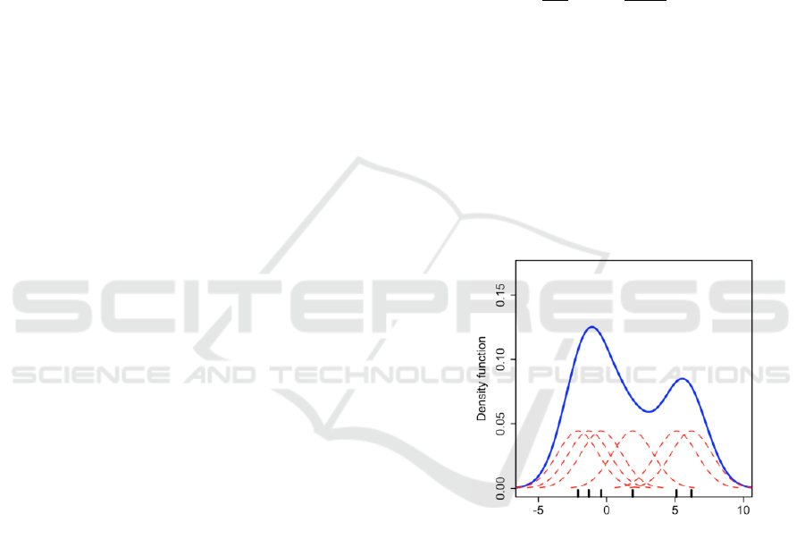
Fig. 1 illustrates a set of data points (black vertical

lines on the x-axis) and their individual kernels (red

lines) computed using Gaussian kernel. The overall

density (blue curve) is computed by summing these

individual functions according to Equation 1.

Figure 1: Kernel density estimate (KDE).

The bandwidth h plays the role of a smoothing scale,

and determines how much emphasis is put on the clos-

est points. It is well recognized that the choice of the

bandwidth is a crucial problem for KDE (Gramacki,

2018). This problem is often known as bandwidth se-

lection.

To illustrate the effect of this hyperparameter , Fig.

2 shows the kernel density estimate of a random sam-

ple of 1000 samples from a Gaussian distribution us-

ing different bandwidth values. As we can see, the

most appropriate estimation has been obtained when

h = 0.22. However, when h is too small, (h = 0.03)

the density is undersmoothed. On the contrast, for a

large value of the bandwidth (h = 1.5), the density is

oversmoothed (Chen, 2017).

Dimensionality Reduction and Bandwidth Selection for Spatial Kernel Discriminant Analysis

279

Figure 2: Kernel density estimate (KDE) with different

bandwidths.

One of the well-known application of Kernel Den-

sity Estimation is its use to build a supervised clas-

siﬁer upon Bayes’ theorem, called Kernel Discrim-

inant Analysis (KDA). In fact, for a training set

of n d-dimensional samples grouped into m classes,

Bayes discriminant rule consists of assigning a d-

dimensional observation x to the class k

with highest

posterior probability, formulated as:

= argmax

k∈{1,2,...,m}

(π

(x)) (2)

Where f

is the probability density function of x in

the class k and π

is the a priori probability that an ob-

servation belongs to the class k(k = 1, ..., m). Kernel

Discriminant Analysis rule consists of using Kernel

Density Estimation (Equation 1) to estimate the the

density functions f

3 SPATIAL KERNEL

DISCRIMINANT ANALYSIS

Like most classiﬁcation algorithms, Kernel Discrim-

inant Analysis assumes that data samples are inde-

pendent and identically distributed (i.i.d). However,

this assumption is often violated in many real-life

problems, for example, in georeferenced data con-

taining a spatial dimension and characterized by spa-

tial autocorrelation phenomena. This characteristic

comes from the fact that more the objects are close

to each other, the higher is the correlation between

them (Miller, 2004).

In (Boumeddane et al., 2019) and (Boumeddane

et al., 2020), the authors proposed an extension of

Kernel Discriminant Analysis (KDA) for spatially de-

pendent data, based on a Spatial Kernel Density Esti-

mator (SKDE) proposed by (Dabo-Niang et al., 2014)

which takes into account the spatial positions of data.

We consider a spatial process {Z

= (X

, Y

) ∈

× [1, m], s ∈ Z

, d ∈ N

∗

, m ∈ N

∗

}, representing a

set of d-dimensional observations x

measured each at

a site (geographic position) s ∈ Z

and y

is the class

label (1...m) to which x

belongs.

Suppose that x

(k)

, x

(k)

, ..., x

(k)

are d-dimensional

observations from the k-th class (k = 1, 2, ..., m) of the

training set (of a total size n), measured at the sites

, s

, ..., s

respectively.

An observation x

∈ R

located at a site s

, will

be assigned to the class k

, where:

= argmax

k∈{1,2,...,m}

(

(x)) (3)

The class density function f

of the k-th class is

estimated using the spatial kernel density estimator

(SKDE) of (Dabo-Niang et al., 2014), deﬁned as:

) =

∑

i=1

− x

(k)



− s



(4)

where:

• h

and h

are two bandwidths controlling, respec-

tively, features and spatial neighbourhood,

• K

and K

are two kernels respectively deﬁned in

and R, where K

manages observations’ values

while K

deals with the spatial dimension of data,

• k s

− s

k is the Euclidean distance between the

sites s

and s

4 RELATED WORK

In literature, a set of data-based bandwidth selec-

tors have been proposed for kernel density estima-

tion. The core idea behind these methods is to ﬁnd

the optimal bandwidth which minimises the Mean In-

tegrated Squared Error (MISE) between the estimated

and actual probability density function (Chen, 2017),

formulated as:

MISE(h) = E[

(

f (x) − f (x))

dx] (5)

These methods include: (1) Rules-of-thumb : such as,

Silverman’s rule of thumb and Scott’s rule of thumb.

These rules rely upon some assumption on the den-

sity, like the assumption of a normal density in Silver-

man’s rule, which makes these methods not totality

data-driven (Zhou et al., 2018) , (2) Cross-validation

based approaches: including least square cross val-

idation, biased cross validation and smoothed cross

validation, (3) Plug-in approaches and (4) Bootstrap

approaches (Chen, 2017).

ICAART 2021 - 13th International Conference on Agents and Artiﬁcial Intelligence

280

These bandwidth selection techniques that aim to

minimise the MISE may note be suitable for classiﬁ-

cation purpose, in other words the optimal bandwidth

that minimise the MISE may not be optimal to min-

imise the misclassiﬁcation rate (Ghosh and Chaud-

huri, 2004). In addition, SKDA depends on two band-

widths related to featutes on one hand, and spatial

neighbourhood on the other hand. These bandwidth

selection methods do not consider the spatial dimen-

sion of data.

Few works has addressed dimensionality reduc-

tion and bandwidth selection for Kernel Discrimi-

nant Analysis. In (Sheikhpour et al., 2016), the au-

thors proposed a hybrid model of Particle Swarm Op-

timization (PSO) and Kernel Discriminant Analysis

using PSO metaheuristic for both features and op-

timal bandwith selection. This model was applied

for breast cancer diagnosis. Moreover, (Baek et al.,

2016) proposed an approach which integrates Ker-

nel Discriminant analysis and the information theo-

retic measure of complexity (ICOMP) with genetic

algorithm (GA), used simultaneously for features and

bandwidth selection. Recently, (Sheikhpour et al.,

2017) proposed a kernelized non-parametric classiﬁer

based on feature ranking in anisotropic Gaussian ker-

nel (KNR-AGK). This approach uses features’ ranks

for both feature selection and parameters learning

of the anisotropic Gaussian kernel, considering these

ranks as the kernel bandwidths of different dimen-

sions.

5 BACKGROUND

In this section we present an overview of the two con-

cepts that we will use in our hybrid method : Principle

Component Analysis and Particle Swarm Optimisa-

tion.

5.1 Principle Component Analysis

Principal component analysis (PCA) is a dimension-

ality reduction technique, which projects a data set

of a high-dimensional space into a lower-dimensional

sub-space, with the goal of preserving most of the

variation. It is a mathematical algorithm, which con-

sists of ﬁnding a linear combination converting the

original variables into a new set of uncorrelated vari-

ables (the principle components) which capture max-

imal variance. PCA can be performed via an eigen

decomposition of the covariance matrix C (d × d) (Pu

et al., 2014), given by:

C = W ΛW

−1

(6)

where:

• W is a (d × d) matrix of eigenvectors, which rep-

resents the principle components,

• and Λ is a diagonal matrix of d eigenvalues.

Principle components are ordered such that ﬁrst

ones has maximum variance. For a dimensionality re-

duction purpose, features with small eigenvalues may

be dismissed and the data points will be projected

onto the ﬁrst k Principle Components (van der Walt

and Barnard, 2017).

5.2 Particle Swarm Optimisation

Particle Swarm Optimisation (PSO) is a nature-

inspired metaheuristic originally proposed by

Kennedy and Elberhart in 1995, that simulates the so-

cial behaviour of some animals such as insects, herds,

schools of ﬁsh or ﬂocks of birds which cooperate to

ﬁnd food. PSO is a population based stochastic opti-

mization technique, which uses a population called

swarm composed of N particles that moves over the

research space, iteration to iteration. Each particle

has a position vector X

, x

, ...., x

) and a velocity

vector v

, v

..., v

), where i ∈ {1, 2, ..., N} and

d is the number of dimensions in the vector. Each

particle represents a potential solution to the problem

in the d-dimensional research space (Wang et al.,

2018).

The optimization process starts with a randomly

initialized population of solutions. During the re-

search process of the optimal solution, each parti-

cle adjust its search direction toward a promising

search region according to its own optimal experi-

ence (pbest

) and the optimal experience of the swarm

(called the global best: gbest). The performance of

each particle is measured using a ﬁtness function re-

lated to the problem deﬁnition.

The velocity and position of each particle are up-

dated using the following equations (Wang et al.,

2018):

i,t+1

= wv

i,t

+ c

i,t

− x

i,t

) +c

g,t

− x

i,t

) (7)

i,t+1

= x

i,t

+ v

i,t+1

(8)

Where: w is the inertia weight, c

and c

are acceler-

ation constants, and r

and r

are uniformly random

values between 0 and 1.

This process is repeated until a stop criteria is sat-

isﬁed, such as a maximum number of iterations.

Dimensionality Reduction and Bandwidth Selection for Spatial Kernel Discriminant Analysis

281

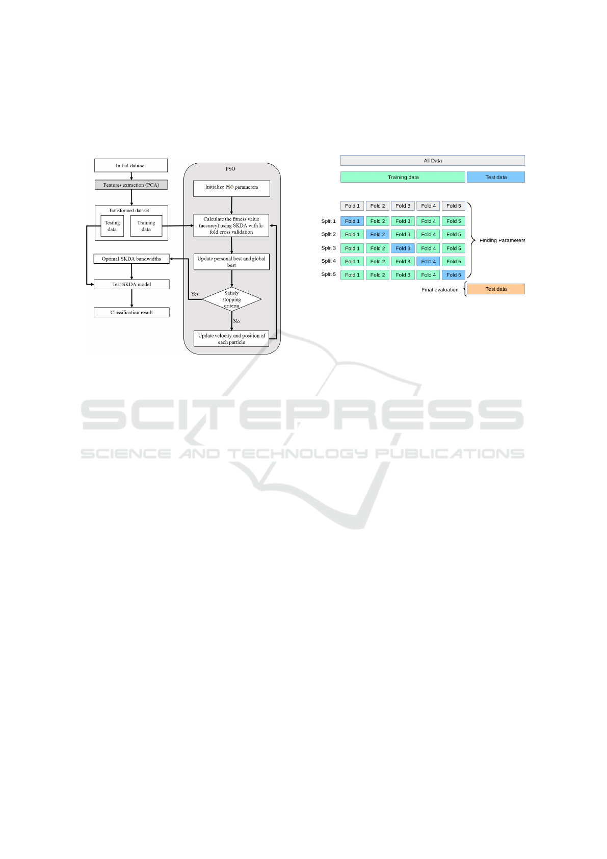
6 PROPOSED APPROACH

We summarize in Fig. 3 the steps of our proposed

approach that we called PSO-SKDA.

Figure 3: PSO-SKDA approach.

Step 1: PCA for Features Extraction. We pro-

pose to apply PCA as a preprocessing step prior to

SKDA. PCA will serves as a dimensionality reduc-

tion technique and also as bandwidth regularizer. As

previously explained, only the ﬁrst principle compo-

nents with highest eigenvalues will be kept. More-

over, we performed PCA on non-spatial dimensions

only, while preserving spatial information. In addi-

tion, we performed PCA on the training set samples,

than apply the same linear transformation on the test

set before the classiﬁcation. The number of selected

principal components will be denoted d

Step 2 : PSO for Bandwidths Selection. In this

step we use PSO technique to carry out the selec-

tion of the optimal values of the bandwidths h

and h

which maximise the classiﬁcation accuracy of SKDA.

That is to say that, we deﬁned the ﬁtness function as

the classiﬁcation overall accuracy of SKDA and band-

width selection consists of ﬁnding the optimal band-

widths which maximise the classiﬁcation accuracy.

Moreover, we encode the solutions as a (d

+ 1) di-

mensional vector H = [hv

, hv

, ..., hv

, h

] where d

is the number of the retained principal components

and hv

is the bandwidth of the i-th feature.

In each iteration of PSO, the objective function is

calculated for all particles using SKDA, based on a

k-fold cross validation on the training set. Figure 4 il-

lustrates the concept of k-fold cross validation, which

consists of splitting the training set into k subsets of

same size and using k −1 folds to train the model and

the remaining fold for validation. The output of the

model is the average of the values computed in the

loop.

Figure 4: k-fold cross validation.

Also, the position of particles are updated using

Equations 7 and 8, and global and per-particle best

solutions are updated.

Step 3: Classiﬁcation with the Optimal Deter-

mined Kernel Bandwidths. The ﬁnal step consists

of the classiﬁcation of the transformed testing data us-

ing SKDA classiﬁer based on the determined optimal

kernel bandwidths.

7 EXPERIMENTS

7.1 Experimental Setup

We applied our approach for Hyperspectral image

classiﬁcation which consists of assigning a label (ex:

water, forest ...) to a pixel. A hyperspectral image

(HSI) is a set of simultaneous images collected for

the same area on the surface of the earth with hun-

dreds of spectral bands at different wavelength chan-

nels and with high resolution. Each pixel of a HSI

at a position s

(representing the spatial dimension) is

characterized by a d-dimensional spectral vector (rep-

resenting the spectral dimension).

These images are characterised by the high num-

ber of spectral bands. Also, from a spectral point

of view, pixels of the same materials have similar

spectral signature (Benediktsson and Ghamisi, 2015).

Moreover, a strong correlation exists between neigh-

bouring bands of a hyperspectral image. This fact

motivates the use of feature selection and feature ex-

traction techniques to reduce the dimensionality of the

ICAART 2021 - 13th International Conference on Agents and Artiﬁcial Intelligence

282

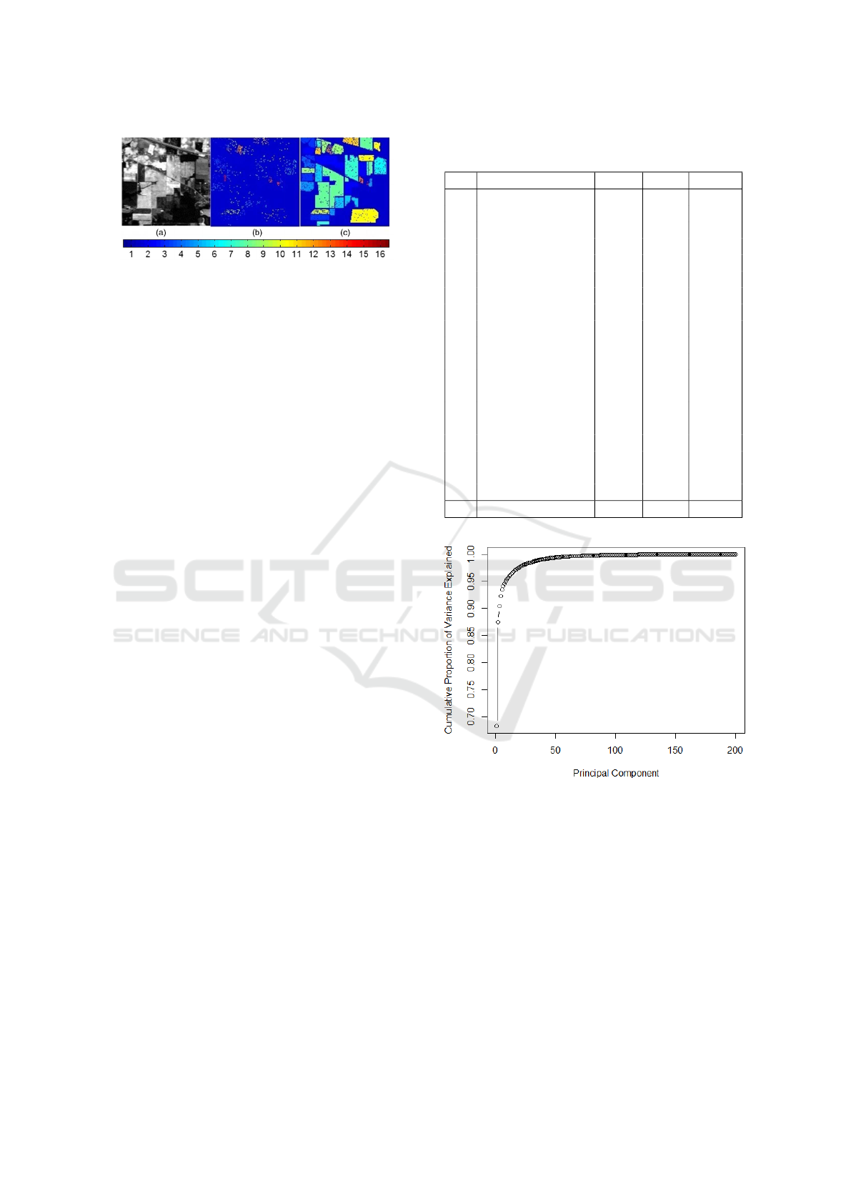
Figure 5: Indian Pines dataset: (a) false color image,

(b) training samples, and (c) test samples (Ghamisi et al.,

2014).

hyperspectral cube.

Moreover, from the spatial perspective, the spec-

tral signatures are spatially correlated, which mean

that neighbouring pixels usually belongs to the same

material especially for high-resolution images. This

characteristic known as spatial autocorrelation should

be taken into account for an effective analysis.

We conducted our experiments on a 200-

dimensional dataset named Indian Pines dataset,

which consists of a 145 × 145 pixels image over

the Indian Pines site in Northwestern Indiana. The

ground truth is classiﬁed into 16 classes, containing

agriculture, forest and natural vegetation. We used

standard training and test sets (Mou et al., 2018),

widely used by the HSI classiﬁcation community.

This makes our results entirely comparable to state-

of-the-art methods. Fig. 5 visualizes this image and

the training and test samples that we used. Table 1

displays the size of each class of this dataset’s train-

ing and testing sets.

To evaluate the performance of our algorithm,

we use the following measures: 1) Average Accu-

racy (AA) : representing the average value of the

class classiﬁcation accuracy (CA). 2) Overall accu-

racy (OA) : which represents the ratio of correctly

classiﬁed samples, i.e. calculated as the number of

correctly classiﬁed pixels, divided by the number of

test samples. 3) Kappa Coefﬁcient (κ) : that pro-

vides information regarding the amount of agreement

corrected by the level of agreement that could be ex-

pected due to chance alone.

7.2 Experimental Results

To decide how much principle components to keep,

while retaining as much of the information as pos-

sible, we use the Cumulative Proportion of Variance

Explained graph (Figure 6). We only keep the trans-

formed features with highest eigenvalues such that the

cumulative proportion of variance explained is about

98%. For the Indian Pines dataset with an original

feature space of 200 variables, only 25 principle com-

ponents are selected.

Table 1: Class labels and the number of training and testing

samples for Indian pines dataset.

Name Train Test Total

1 Corn-no till 50 1384 1434

2 Corn-min till 50 784 834

3 Corn 50 184 234

4 Grass-pasture 50 447 497

5 Grass-trees 50 697 747

6 Hay-windrowed 50 439 489

7 Soybean-no till 50 918 968

8 Soybean-min till 50 2418 2468

9 Soybean-clean 50 564 614

10 Wheat 50 162 212

11 Woods 50 1244 1294

12 Bldg-grass-tree-

drives

50 330 380

13 Stone-Steel-

Towers

50 45 95

14 Alfalfa 15 39 54

15 Grass-pasture-

mowed

15 11 26

16 Oats 15 5 20

Total 695 9671 10366

Figure 6: Cumulative Proportion of Variance Explained

graph for IP dataset.

Moreover, we executed the PSO process to select

the optimal bandwidth with 20 iterations where each

swarm contains 20 particles. Using a 5-fold cross-

validation and an Epanechnikov kernel for K

and K

The parameters of PSO are initialized as follows:

= c

= 1.93 , w = 0.72. Also, the solution space is

reduced to the values between 1 and 10.

Using our approach, the best solutions found are:

= 6 and h

= 3.5, here we used same h

for all

feature dimensions.

We compared PSO-SKDA results to state-of-the-

art techniques related to Hyperspectral images classi-

Dimensionality Reduction and Bandwidth Selection for Spatial Kernel Discriminant Analysis

283

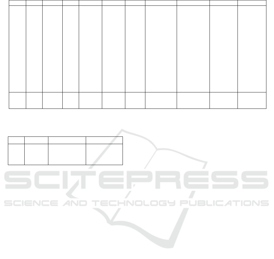
Table 2: Classiﬁcation results (%) for Indian Pines dataset using standard training and test sets.

SVM RF-200 RNN 1D-CNN 2D-CNN SICNN Res. C-D Net RNN-GRU-Pr SSCasRNN PSO-SKDA

CA1 64.31 54.84 64.74 61.34 82.51 79.84 74.86 70.59 86.99 89.74

CA2 70.92 58.42 61.35 60.33 88.14 92.47 95.28 70.82 98.72 97.07

CA3 84.78 82.61 74.46 80.43 100.0 99.46 100.0 81.52 100.0 100.0

CA4 91.05 85.91 83.45 89.04 94.85 93.29 95.08 90.16 94.41 88.14

CA5 85.94 80.49 77.04 90.53 85.80 92.68 96.56 91.97 97.42 95.84

CA6 93.62 94.76 87.70 96.13 99.77 96.58 99.09 96.13 100.0 99.77

CA7 69.17 77.34 76.03 72.11 82.35 86.82 84.42 84.75 87.15 90.63

CA8 52.90 59.43 60.79 54.47 73.86 69.52 74.57 59.64 85.98 85.98

CA9 76.60 63.48 61.17 75.71 86.00 83.69 80.14 86.17 87.23 88.30

CA10 97.53 96.06 93.21 99.83 100.0 100.0 100.0 99.38 100.0 99.38

CA11 77.49 88.26 81.67 80.87 94.53 96.70 95.74 84.97 97.51 98.07

CA12 73.33 54.85 55.45 78.48 97.27 96.97 96.06 77.58 99.70 99.09

CA13 100.0 97.78 86.67 91.11 100.0 100.0 100.0 95.56 100.0 100.0

CA14 87.18 58.97 69.23 94.87 97.44 94.87 84.62 84.62 100.0 100.0

CA15 90.91 81.82 90.91 90.91 100.0 100.0 100.0 90.91 100.0 100.0

CA16 100.0 100.0 80.00 100.0 100.0 100.0 100.0 100.0 100.0 100.0

OA 70.55 69.79 69.82 70.79 85.43 85.13 85.76 88.63 91.79 92.07

AA 82.23 77.13 75.24 82.23 92.66 92.68 92.28 85.63 95.79 95.75

κ 66.90 65.89 65.87 67.07 83.49 83.13 83.85 73.66 90.62 90.94

Table 3: Comparaison between SKDA, PCA-SKDA and

PSO-SKDA for Indian Pines dataset.

SKDA PCA-SKDA PSO-SKDA

OA 93.89 92.71 92.07

AA 96.67 96.13 95.75

κ 93.01 98.18 90.94

ﬁcation, including: SVM, RF-200 which consists of

a Random forest with 200 trees, RNN, 1D CNN, 2D

CNN, SICNN, Res. Conv-Deconv Net (Mou et al.,

2018), RNN-GRU-PRetanh (Mou et al., 2017) and

SSCasRNN (Hang et al., 2019).

Since we use same sets of training and test, we

reported the results of SVM, RNN, 1D-CNN and 2D-

CNN from (Hang et al., 2019). In addition, the re-

sults of RF-200 and RNN-GRU-PRetanh are reported

from (Mou et al., 2017). Finally, those of SICNN and

Res. Conv-Deconv Net are reported from (Mou et al.,

2018).

Table 2 shows classiﬁcation results of Indian pines

dataset. As we might notice, PSO-SKDA gives com-

petitive classiﬁcation accuracies comparing to state-

of-the art methods with highest overall accuracy and

kappa coefﬁcient. PSO-SKDA gives best or equiva-

lent results for 10 classes from 16, with a 100% accu-

racy for 5 classes. This experiment shows the effec-

tiveness of the proposed method, and that dimension-

ality reduction using PCA didn’t affected the accuracy

of our classiﬁer. In addition, even with limited num-

ber of training set, the hypermatametrs tuning from

the training set gave good results on the new values of

the test set.

In Table 3, we compare the results of PSO-SKDA

to SKDA (Boumeddane et al., 2020) and PCA-SKDA

where the bandwidths where tuned experimentally us-

ing a grid search like approach based on test set.

This results shows that our new approach PSO-

SKDA is more accurate then SKDA and PCA-SKDA.

In fact, the results of these two approaches are over-

estimated since the test set was used for the hyperpa-

rameters tuning, this introduces a bias in the results.

8 CONCLUSION

In this paper, we introduced a new hybrid approach,

which integrates Spatial Kernel Discriminant Anal-

ysis, Principle Components Analysis and Particle

Swarm Optimisation. This model aims to automate

the choice of the optimal values of the bandwidths

an d h

and reduce the computational complex-

ity due to the high dimensionality of data. Exper-

iments on Hyperspectral Image classiﬁcation have

shown promising results of PSO-SKDA on Indian

Pines dataset compared to latest state-of-the-art algo-

rithms for HSI classiﬁcation. As a future work, we

aim to validate our approach on other datasets and to

enhance the execution time which remains problem-

atic for kernel density estimation based algorithms es-

pecially for huge datasets. This issue needs more in-

vestigation to improve the computational complexity.

REFERENCES

Baek, S. H., Park, D. H., and Bozdogan, H. (2016). Hy-

brid kernel density estimation for discriminant anal-

ysis with information complexity and genetic algo-

rithm. Knowl.-Based Syst., 99:79–91.

Benediktsson, J. A. and Ghamisi, P. (2015). Spectral-spatial

ICAART 2021 - 13th International Conference on Agents and Artiﬁcial Intelligence

284

classiﬁcation of hyperspectral remote sensing images.

Artech House.

Boumeddane, S., Hamdad, L., Dabo-Niang, S., and Had-

dadou, H. (2019). Spatial kernel discriminant anal-

ysis: Applied for hyperspectral image classiﬁcation.

In Proceedings of the 11th International Conference

on Agents and Artiﬁcial Intelligence, ICAART 2019,

Volume 2, Prague, Czech Republic, February 19-21,

2019., pages 184–191.

Boumeddane, S., Hamdad, L., Haddadou, H., and Dabo-

Niang, S. (2020). A kernel discriminant analysis for

spatially dependent data. Distributed and Parallel

Databases, pages 1–24.

Chen, Y.-C. (2017). A tutorial on kernel density estimation

and recent advances. Biostatistics & Epidemiology,

1(1):161–187.

Dabo-Niang, S., Hamdad, L., Ternynck, C., and Yao, A.-

F. (2014). A kernel spatial density estimation allow-

ing for the analysis of spatial clustering. application

to monsoon asia drought atlas data. Stochastic envi-

ronmental research and risk assessment, 28(8):2075–

2099.

Ghamisi, P., Benediktsson, J. A., Cavallaro, G., and Plaza,

A. (2014). Automatic framework for spectral-spatial

classiﬁcation based on supervised feature extraction

and morphological attribute proﬁles. IEEE J. Sel. Top.

Appl. Earth Obs. Remote. Sens., 7(6):2147–2160.

Ghosh, A. K. and Chaudhuri, P. (2004). Optimal smooth-

ing in kernel discriminant analysis. Statistica Sinica,

pages 457–483.

Gramacki, A. (2018). Nonparametric kernel density esti-

mation and its computational aspects. Springer.

Hang, R., Liu, Q., Hong, D., and Ghamisi, P. (2019). Cas-

caded recurrent neural networks for hyperspectral im-

age classiﬁcation. IEEE Trans. Geoscience and Re-

mote Sensing, 57(8):5384–5394.

Li, J., Cheng, K., Wang, S., Morstatter, F., Trevino, R. P.,

Tang, J., and Liu, H. (2018). Feature selection: A data

perspective. ACM Comput. Surv., 50(6):94:1–94:45.

Miller, H. J. (2004). Tobler’s ﬁrst law and spatial analysis.

Annals of the Association of American Geographers,

94(2):284–289.

Mou, L., Ghamisi, P., and Zhu, X. X. (2017). Deep recur-

rent neural networks for hyperspectral image classiﬁ-

cation. IEEE Trans. Geoscience and Remote Sensing,

55(7):3639–3655.

Mou, L., Ghamisi, P., and Zhu, X. X. (2018). Un-

supervised spectral-spatial feature learning via deep

residual conv-deconv network for hyperspectral image

classiﬁcation. IEEE Trans. Geoscience and Remote

Sensing, 56(1):391–406.

Pu, H., Chen, Z., Wang, B., and Jiang, G.-M. (2014). A

novel spatial–spectral similarity measure for dimen-

sionality reduction and classiﬁcation of hyperspectral

imagery. IEEE Transactions on Geoscience and Re-

mote Sensing, 52(11):7008–7022.

Sheikhpour, R., Sarram, M. A., Chahooki, M. A. Z., and

Sheikhpour, R. (2017). A kernelized non-parametric

classiﬁer based on feature ranking in anisotropic gaus-

sian kernel. Neurocomputing, 267:545–555.

Sheikhpour, R., Sarram, M. A., and Sheikhpour, R. (2016).

Particle swarm optimization for bandwidth determina-

tion and feature selection of kernel density estimation

based classiﬁers in diagnosis of breast cancer. Appl.

Soft Comput., 40:113–131.

Silverman, B. W. (1986). Density estimation for statistics

and data analysis, volume 26. CRC press.

van der Walt, C. M. and Barnard, E. (2017). Variable

kernel density estimation in high-dimensional feature

spaces. In Proceedings of the Thirty-First AAAI Con-

ference on Artiﬁcial Intelligence, February 4-9, 2017,

San Francisco, California, USA., pages 2674–2680.

Wang, D., Tan, D., and Liu, L. (2018). Particle swarm op-

timization algorithm: an overview. Soft Computing,

22(2):387–408.

Zaman, F., Wong, Y., and Ng, B. (2016). Density-based

denoising of point cloud. CoRR, abs/1602.05312.

Zhou, Z., Si, G., Zhang, Y., and Zheng, K. (2018). Robust

clustering by identifying the veins of clusters based on

kernel density estimation. Knowledge-Based Systems,

159:309–320.

Dimensionality Reduction and Bandwidth Selection for Spatial Kernel Discriminant Analysis

285