EasyPBR: A Lightweight Physically-based Renderer

Radu Alexandru Rosu

and Sven Behnke

Autonomous Intelligent Systems, University of Bonn, Germany

Keywords:

Physically-based Rendering, Synthetic Data Generation, Visualization Toolkit.

Abstract:

Modern rendering libraries provide unprecedented realism, producing real-time photorealistic 3D graphics on

commodity hardware. Visual ﬁdelity, however, comes at the cost of increased complexity and difﬁculty of

usage, with many rendering parameters requiring a deep understanding of the pipeline. We propose EasyPBR

as an alternative rendering library that strikes a balance between ease-of-use and visual quality. EasyPBR con-

sists of a deferred renderer that implements recent state-of-the-art approaches in physically based rendering.

It offers an easy-to-use Python and C++ interface that allows high-quality images to be created in only a few

lines of code or directly through a graphical user interface. The user can choose between fully controlling the

rendering pipeline or letting EasyPBR automatically infer the best parameters based on the current scene com-

position. The EasyPBR library can help the community to more easily leverage the power of current GPUs to

create realistic images. These can then be used as synthetic data for deep learning or for creating animations

for academic purposes.

1 INTRODUCTION

Modern rendering techniques have become advanced

enough for photorealistic images to be produced even

on commodity hardware. Advances such as real-time

ray tracing and physically-based materials have al-

lowed current rendering pipelines to closely follow

the theoretical understanding of light propagation and

how it interacts with the real world. However, such

advancements in rendering come with an increase in

complexity for the end user, often requiring a deep un-

derstanding of the rendering pipeline to achieve good

results

†

Our proposed EasyPBR addresses this issue by of-

fering a 3D viewer for visualizing various types of

data (meshes, point clouds, surfels, etc.) with high-

quality renderings while maintaining a low barrier of

entry. Scene setup and object manipulation can be

done either through Python or C++. Furthermore,

meshes can be manipulated through the powerful li-

https://orcid.org/0000-0001-7349-4126

https://orcid.org/0000-0002-5040-7525

†

This work has been funded by the Deutsche

Forschungsgemeinschaft (DFG, German Research Founda-

tion) under Germany’s Excellence Strategy - EXC 2070 -

390732324 and by the German Federal Ministry of Educa-

tion and Research (BMBF) in the project Kompetenzzen-

trum: Aufbau des Deutschen Rettungsrobotik-Zentrums

(A-DRZ).

bigl (Jacobson et al., 2018) library for geometry pro-

cessing since our mesh representation shares a com-

mon interface. The user can choose to conﬁgure ren-

dering parameters before the scene setup or at runtime

through the GUI. If the parameters are left untouched,

EasyPBR will try to infer them in order to best ren-

der the given scene. EasyPBR uses state-of-the-art

rendering techniques and offers easy extensions for

implementing novel methods through using a thin ab-

straction layer on top of OpenGL.

EasyPBR and all the code needed to reproduce the

ﬁgures in this paper is made available at

https://github.com/AIS-Bonn/easy pbr

A video with additional footage is also available on-

line

Our main contributions are:

• a lightweight framework for real-time physically-

based rendering,

• an easy-to-use Python front-end for scene setup

and manipulation, and

• powerful mesh manipulation tools through the li-

bigl (Jacobson et al., 2018) library.

http://www.ais.uni-bonn.de/videos/GRAPP 2020

Rosu/

Rosu, R. and Behnke, S.

EasyPBR: A Lightweight Physically-based Renderer.

DOI: 10.5220/0010268902450252

In Proceedings of the 16th International Joint Conference on Computer Vision, Imaging and Computer Graphics Theory and Applications (VISIGRAPP 2021) - Volume 1: GRAPP, pages

245-252

ISBN: 978-989-758-488-6

245

2 RELATED WORK

Various 3D libraries currently offer rendering of high

ﬁdelity visuals. Here we compare against the most

widely used ones.

Meshlab (Cignoni et al., 2008) is a popular open-

source tool for processing, editing, and visualizing

triangular meshes. Its functionality can be accessed

either through the graphical user interface (GUI) or

the provided scripting interface. This makes Mesh-

lab difﬁcult to integrate into current Python or C++

projects. In contrast, EasyPBR offers both a Python

package that can be easily imported and a shared li-

brary that can be linked into an existing C++ project.

EasyPBR also integrates with libigl (Jacobson et al.,

2018), allowing the user to access powerful tools

for geometry processing. Additionally, EasyPBR of-

fers more realistic renderings of meshes together with

functionality for creating high-resolution screenshots

or videos.

Blender (Blender Online Community, 2018) is an

open-source 3D creation suite. It includes all aspects

of 3D creation, from modeling to rendering and video

editing; and it offers a Python API, which can be used

for scripting. However, the main usage of Blender

is to create high-quality visuals through ray-traced

rendering, which is far from real-time capable. The

Python API is also not the main intended use case of

Blender, and while rendering commands can be is-

sued through scripts, there is no visual feedback dur-

ing the process. In contrast, we offer real-time ren-

dering and control over the scene from small Python

or C++ scripts.

VTK (Schroeder et al., 2000) is an open-source

scientiﬁc analysis and visualization tool. While ini-

tially its main rendering method was based on Phong

shading, recently a physically-based renderer together

with image-based lighting (IBL) has also been in-

cluded. Extensions of the main rendering model with

new techniques is cumbersome as it requires exten-

sive knowledge of the VTK framework. In contrast,

our rendering methods are easy to use and we keep a

thin layer of abstraction on top of OpenGL for simple

extendibility using custom callbacks.

Marmoset toolbag(Marmoset, 2020) is a visual

tool designed to showcase 3D art. It features a real-

time PBR renderer, which allows easy setup of a

scene to create high-quality 3D presentations. How-

ever, it is not available on Linux and is also distributed

under a paid license.

Unreal Engine (Epic Games, 2007) is a state-of-

the-art engine created with the goal to provide real-

time high-ﬁdelity visuals. It has been used in profes-

sional game-making, architecture visualization, and

a) Marmoset

(Marmoset, 2020)

b) EasyPBR

(Ours)

c) VTK

(Schroeder et al., 2000)

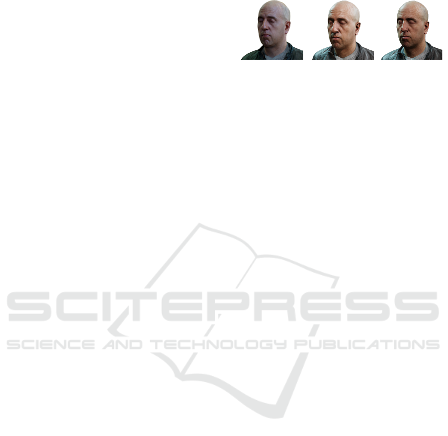
Figure 1: Comparison of various PBR rendering tools.

VR experiences. While it provides a plethora of tools

for content creation, the entry barriers can also be

quite high. Additionally, the Python API provided

can only be used as an internal tool for scripting and

results in cumbersome setup code for even easy im-

porting of assets and rendering. In contrast, EasyPBR

acts as a Python library that can be readily imported

in any existing project and used to draw to screen in

only a couple of lines of code.

We showcase results from EasyPBR compared

with VTK and Marmoset in Fig. 1. We use the high-

quality 3D scan from (3D Scan Store, 2020) and ren-

der it under similar setups. While our renderer does

not feature sub-surface scattering shaders like Mar-

moset, it can still achieve high-quality results in less

than 10 lines of code. In contrast, for similar results,

VTK requires more than 150 lines in which the user

needs to manually deﬁne rendering passes for effects

such as shadows baking and shadow mapping.

3 PHYSICALLY-BASED

RENDERING

Physically-based rendering or PBR is a set of shading

models designed to achieve high realism though accu-

rately modeling light and material interaction. Previ-

ous shading models like Phong shading are not based

on mathematically rigorous analysis of light and can

lead to unrealistic results. PBR attempts to address

this issue by basing the shading equations on the laws

of light interaction.

PBR follows the mathematical modeling of light

based on the reﬂectance equation:

(p, ω

) =

Ω

(p, ω

, ω

(p, ω

)(n· ω

)dω

, (1)

where L

(p, ω

) is the outgoing radiance from point

p in direction ω

which gathers over the hemisphere

Ω the incoming radiance L

weighted by the BRDF

(p, ω

, ω

) and the angle of incidence between the

incoming ray ω

and the surface normal n.

To model materials in a PBR framework we use

the Cook-Torrance (Cook and Torrance, 1982) BRDF.

GRAPP 2021 - 16th International Conference on Computer Graphics Theory and Applications

246

Material properties are speciﬁed by two main param-

eters: metalness and roughness. These parameters

cover the vast majority of the real-world materials.

By using a physically-based renderer, they will look

realistic under different illumination conditions.

Since Cook-Torrance is just an approximation of

the underlying physics and there are many variants

used in literature, some more realistic, others more

efﬁcient, we choose the same approximation used in

Unreal Engine 4 (Karis, 2013) which strikes a good

balance between realism and efﬁciency.

3.1 Image-based Lighting

To fully solve the reﬂectance equation, light incom-

ing onto the surface would have to be integrated over

the whole hemisphere. However, this integral is not

tractable in practice, and therefore, one approxima-

tion would be to gather only the direct contributions

of the light sources in the scene. This has the un-

desirable effect of neglecting secondary bounces of

light and causing shadows to be overly dark, yield-

ing a non-realistic appearance. To address this, we

use image-based lighting, which consists of embed-

ding our 3D scene inside a high dynamic range (HDR)

environment cubemap in which every pixel acts as a

source of light. This greatly enhances the realism of

the scene and gives a sense that our 3D models ”be-

long” in a certain environment as changes in the HDR

cubemap have a visible effect on the model’s lighting.

Efﬁcient sampling of the radiance from the envi-

ronment map is done through precomputing increas-

ingly blurrier versions of the cubemap, allowing for

efﬁcient sampling at runtime of only one texel that

corresponds with a radiance over a large region of

the environment map. Specular reﬂections are also

precomputed using the split-sum approximation. For

more detail, we refer to the excellent article from Epic

Games (Karis, 2013).

We further extend the IBL by implementing the

approach of (Fdez-Ag

uera, 2019) which further im-

proves the visual quality of materials by taking into

account multiple scatterings of light with only a slight

overhead in performance.

4 DEFERRED RENDERING

Rendering methods are often divided in two groups:

forward rendering and deferred rendering, both with

different pros and cons.

Forward rendering works by rendering the whole

scene in one pass, projecting every triangle to the

Final

Metal and rough

Albedo

SSAO

Normals

Figure 2: The various G-Buffer channels together with Am-

bient Occlusion are composed into one ﬁnal texture to be

displayed on the screen. Here we display slices of each

channel that is used for compositing.

screen and shading in one render call. This has the ad-

vantage of being simple to implement but may suffer

from overdraw as having a lot of overlapping geome-

try causes much wasted effort in shading and lighting.

Deferred rendering attempts to solve this issue by

delaying the shading of the scene to a second step.

The ﬁrst step of a deferred renderer writes the mate-

rial properties of the scene into a screen-size buffer

called the G-Buffer. The G-Buffer typically records

the position of the fragments, color, and normal. A

second rendering pass reads the information from the

G-Buffer and performs the light calculations. This

has the advantage of performing costly shading oper-

ations only for the pixels that will actually be visible

in the ﬁnal image.

EasyPBR uses deferred rendering as its perfor-

mance scales well with an increasing number of

lights. Additionally, various post-processing effects

like screen-space ambient occlusion (SSAO) are eas-

ier to implement in a deferred renderer than a forward

one since all the screen-space information is already

available in the G-Buffer.

Table 1: We structure the G-Buffer into four render targets.

Usage

Format

R G B A

RT0 RGBA8 Albedo Weight

RT1 RGB8 Normals Unused

RT2 RG8 Metal Rough Unused

RT3 R32 Depth Unused

The layout of our G-Buffer is described in Tab. 1.

Please note that in our implementation, we do not

store the position of each fragment but rather store

only the depth map as a ﬂoating-point texture and

reconstruct the position from the depth value. This

saves us from storing three ﬂoat values for the posi-

tion, heavily reducing the memory bandwidth require-

EasyPBR: A Lightweight Physically-based Renderer

247

ments for writing and reading into the G-Buffer. We

additionally store a weight value in the alpha chan-

nel of the ﬁrst texture. This will be useful later when

we render surfels which splat and accumulate onto the

screen with varying weights. Several channels in the

G-Buffer are purposely left empty so that they can be

used for further rendering passes.

A visualization of the various rendering passes

and the ﬁnal composed image is shown in Fig. 2.

4.1 Object Representation

We represent objects in our 3D scene as a series of

matrices containing per-vertex information and pos-

sible connectivity to create lines and triangles. The

following matrices can be populated:

• V ∈ R

(n×3)

vertex positions,

• N ∈ R

(n×3)

per-vertex normals,

• C ∈ R

(n×3)

per-vertex colors,

• T ∈ R

(n×3)

per-vertex tangent vectors,

• B ∈ R

(n×1)

per-vertex bi-tangent vector length,

• F ∈ Z

(n×3)

triangle indices for mesh rendering,

• E ∈ Z

(n×2)

edge indices for line rendering.

Note that for the bi-tangent vector, we store only the

length, as the direction can be recovered through a

cross product between the normal and the tangent.

This saves signiﬁcant memory bandwidth and is faster

than storing the full vector.

4.2 Mesh Rendering

Mesh rendering follows the general deferred render-

ing pipeline. The viewer iterates through the meshes

in the scene and writes their attributes into the G-

Buffer. The attributes used depend on the selected

visualization mode for the mesh (either solid color,

per-vertex color, or texture).

When the G-Buffer pass is ﬁnished, we run a sec-

ond pass which reads from the created buffer and cre-

ates any effect textures that might be needed (SSAO,

bloom, shadows, etc.).

A third and ﬁnal pass is afterwards run which

composes all the effect textures and the G-Buffer into

the ﬁnal image using PBR and IBL.

4.3 Point Cloud Rendering

Point cloud rendering is similar to mesh rendering,

i.e. the attributes of the point cloud are written into

the G-Buffer.

The difference lies in the compositing phase

where PBR and IBL cannot be applied due to the lack

a) Plain cloud b) EDL c) EDL + SSAO

Figure 3: a) plain rendered point clouds results in ﬂat shad-

ing and conveys little information. b) enabling Eye Dome

Lighting gives a slight perception of depth, allowing the

user to distinguish between various shapes. c) adding also

Ambient Occlusion enhances the effect even further.

of normal information. Instead, we rely on eye dome

lighting (EDL) (Boucheny and Ribes, 2011), which

is a non-realistic rendering technique used to improve

depth perception. The only information needed for

EDL is a depth map. EDL works by looking at the

depth of adjacent pixels in screen space and darken-

ing the pixels which exhibit a sudden change of depth

in their neighborhood. The bigger the local difference

in depth values is, the darker the color is. The effect

of EDL can be seen in Fig. 3.

Additionally, by sacriﬁcing a bit more perfor-

mance, the user can also enable SSAO which further

enhances the depth perception by darkening crevices

in the model.

4.4 Surfel Rendering

In various applications like simultaneous localiza-

tion and mapping (SLAM) or 3D reconstruction, a

common representation of the world is through sur-

fels (Droeschel et al., 2017; St

uckler and Behnke,

2014). Surfels are modeled as oriented disks with

an ellipsoidal shape, and they can be used to model

shapes that lack connectivity information. Rendering

surfaces through surfels is done with splatting, which

accumulates in screen space the contributions of var-

ious overlapping surfels. The three-step process of

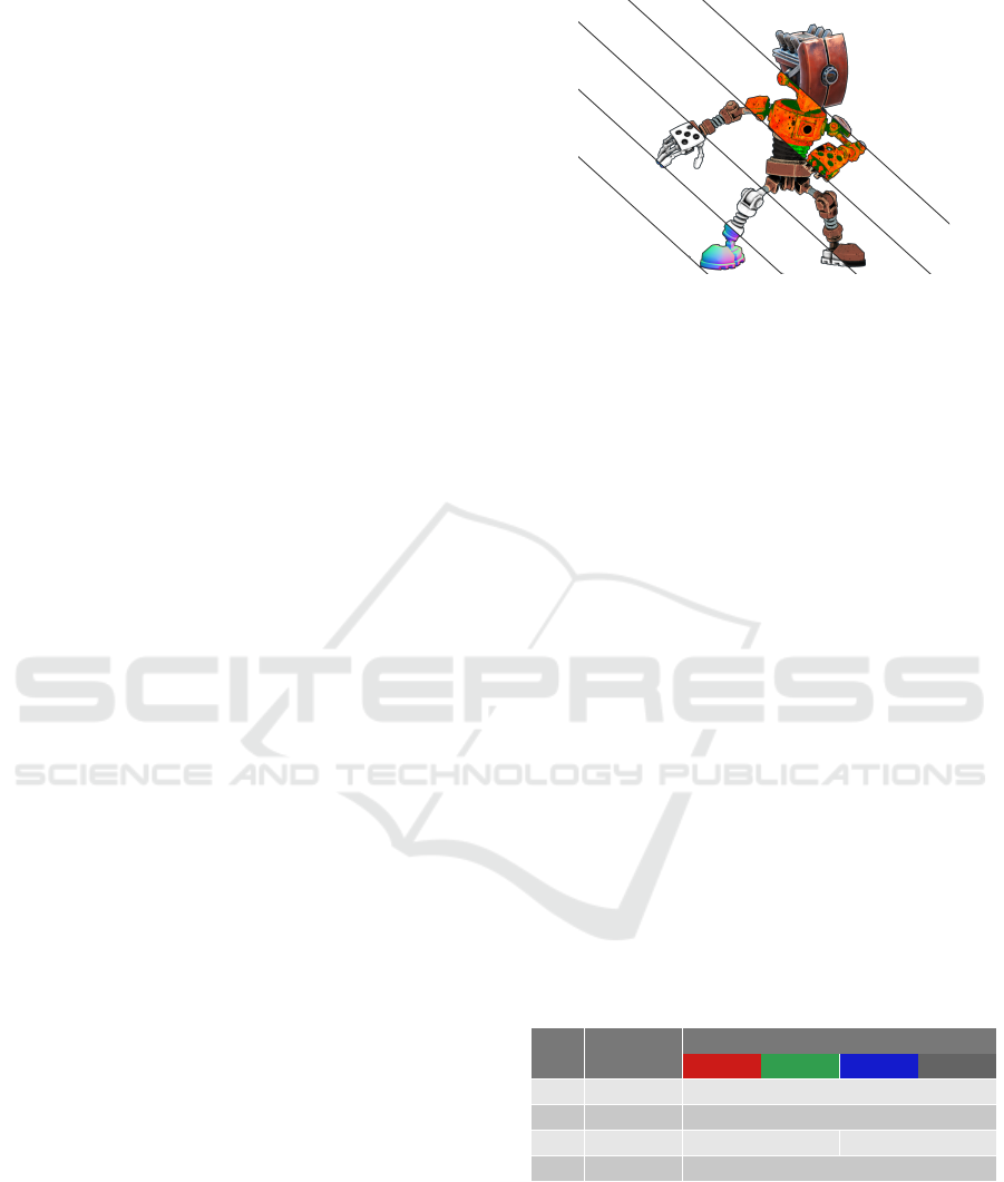
creating the surfels is ilustrated in Fig. 4.

a) b) c)

Figure 4: Surfel rendering is done in three steps. a) the

vertex shader creates a basis from the normal, tangent and

bitangent vectors. b) the geometry shader creates from each

vertex a rectangle orientated according to the basis. c) the

fragment shader creates the elliptical shape by discarding

the fragments in the corners of the rectangle.

GRAPP 2021 - 16th International Conference on Computer Graphics Theory and Applications

248

Figure 5: Comparison between mesh and surfel render-

ing. For clarity, we reduce the radius of the surfels in the

zoomed-in view.

Once the surfels are created, they are rendered into

the G-Buffer. Surfels that overlap within a small dis-

tance to each other accumulate their attributes and in-

crement a weight for the current pixels that will be

used later for normalization.

During surfel rendering, the G-Buffer is changed

from being stored as unsigned bytes to half ﬂoats in

order to support the accumulation of attributes for

overlapping surfels.

The composing pass then normalizes the G-Buffer

by dividing the accumulated albedo, normals, metal-

ness and roughness by the weight stored in the alpha

channel of the albedo.

Finally, composing proceeds as before with the

PBR and IBL pipeline. This yields similar results as

mesh rendering which can be seen in Fig. 5.

4.5 Line Rendering

Line rendering is useful for showing the wireframe

of meshes or for displaying edges between arbitrary

vertices indicated by the E matrix. We perform line

rendering by forward rendering directly into the ﬁnal

image as we do not want lines to be affected by light-

ing and shadowing effects.

5 EFFECTS

Multiple post-processing effects that are supported in

EasyPBR: shadows, SSAO, bloom.

5.1 Shadows

EasyPBR supports point-lights, which can cast

realistic soft shadows onto the scene. Shadows

computation is performed through shadow map-

ping (Williams, 1978). The process works by ﬁrst

rendering the scene only as a depth map into each

point-light as if they were a normal camera.

Afterwards, during compositing, we check if a

fragment’s depth is greater than the depth recorded by

a certain light. If it is greater, then the fragment lies

behind the surface lit by the light and is therefore in

shadow. In order to render soft shadows, we perform

a) Shadows and SSAO b) Bloom

Figure 6: Various post-processing effects can be enabled in

the renderer. Soft shadows and ambient occlusion convey

a sense of depth, and bloom simulates the light bleed from

bright parts of the scene like the sun or reﬂective surfaces.

Percentage Closer Filtering (Reeves et al., 1987) by

checking not only the depth around the current frag-

ment but also the neighboring ones in a 3 × 3 patch

in order to obtain a proportion of how much of the

surface is shadowed instead of just a binary value.

The shadow maps are updated only if the objects

in the scene or the lights move. While the scene re-

mains static, we use the last rendered depth map for

each light. This constitutes a signiﬁcant speed-up

in contrast to the naive approach of recomputing the

shadow map at every frame.

Shadows from multiple lights interacting with the

scene can be observed in Fig. 6a.

5.2 Screen-space Ambient Occlusion

Ambient occlusion is used to simulate the shadowing

effect caused by objects blocking the ambient light.

Simulating occlusion requires global information of

the scene geometry and is usually performed through

ray-tracing, which is costly to compute. Screen-space

ambient occlusion addresses this issue by using only

the current depth buffer as an approximation of the

scene geometry, therefore avoiding the use of costly

global information and making the ambient occlusion

real-time capable. The effect of SSAO can be viewed

in Fig. 6a.

Our SSAO implementation is based on the

Normal-oriented Hemisphere method (Bavoil and

Sainz, 2008). After creating the G-Buffer, we run the

SSAO pass in which we randomly take samples along

the hemisphere placed at each pixel location and ori-

entated according to the normal stored in the buffer.

The samples are compared with the depth buffer in

order to get a proxy of how much the surface is oc-

cluded by neighboring geometry. The SSAO effect is

computed at half the resolution of the G-Buffer and

bilaterally blurred in order to remove high-frequency

noise caused by the low sample count.

EasyPBR: A Lightweight Physically-based Renderer

249

5.3 Bloom

Bloom is the process by which bright areas of the im-

ages bleed their color onto adjacent pixels. This can

be observed, for example, with very bright sunlight,

which causes the nearby parts of the image to increase

in brightness. Bloom is implemented by rendering

into a bright-map only the parts of the scene that are

above a certain level of brightness.

This bright map would now need to be blurred

with a Gaussian kernel and then added on top of the

original image. However, performing blurring at the

resolution of the full screen is too expensive for real-

time purposes, and we, therefore, rely on approxima-

tions. We create an image pyramid with up to six lev-

els from the bright map. We blur each pyramid level

starting from the second one upwards. Blurring by

using an image pyramid allows us to use very large

kernels.

Finally, the bright-map pyramid is added on top of

the original image in order to create a halo-like effect.

The result can be seen in Fig. 6b.

5.4 Final Compositing

The compositing is the ﬁnal rendering pass before

showing the image to the screen. It takes all the pre-

vious rendering passes (G-Buffer, SSAO, etc.) and

combines them to create the ﬁnal image. Finally,

after creating the composed image, it needs to be

tone-mapped and gamma-corrected in order to bring

the HDR values into a low dynamic range (LDR)

range displayable on the screen. For this, we use the

Academy Color Encoding System (ACES) tone map-

per due to its high-quality ﬁlmic look. We further of-

fer support for the Reinhard (Reinhard et al., 2002)

tone mapper.

6 AUTOMATIC PARAMETERS

Various parameters govern the rendering process. The

user can leave them untouched, and our rendering tool

will try to make an educated guess for them at run-

time.

By default, EasyPBR creates a 3-point light setup

consisting of a key light that provides most of the light

for the scene, a ﬁll light softening the shadows, and a

rim light placed behind the object to separate it from

the background. The distances from the object center

towards the light are determined such that the scene

radiance at the object has a predeﬁned value. This

makes the lighting setup agnostic to scaling of the

mesh, so EasyPBR can out of the box render any kind

Table 2: Timings in milliseconds to render a frame.

EasyPBR VTK

Meshlab

v2020.09

Meshlab

v1.3.2

Goliath 6.2 6.1 6.0 558

Head 1.6 1.6 1.1 1.1

of mesh regardless of the unit system it uses. At any

point at runtime, the user can tweak the position, in-

tensity, and color of the lights.

The camera is placed in the world so that the entire

object is in view. Also, the near and far planes of the

cameras are set according to the scale of the scene.

SSAO radius is a function of the scene scale. By

default, we choose the radius to be 5% of the scale of

the scene to be rendered.

The rendering mode depends on the object in the

scene. If the object has no connectivity provided as

triangles in the F matrix, then we render it as a point

cloud using EDL. Otherwise, we render it as a mesh.

If the user provides normals and tangent vectors, then

we render it as a series of surfels. This ensures that

whatever data we put in, our objects will be visualized

in an appropriate manner.

7 PERFORMANCE

We evaluate the performance of EasyPBR and com-

pare it to Meshlab and VTK, as they are common

tools used for visualization. We run all three tools on

an Nvidia RTX 2060. As a metric, we use the mil-

liseconds per frame and test with two meshes, one

high-resolution mesh with 23 million faces (Goliath

statue from Fig. 10) and the 3D scanned head (Fig. 1)

with half a million faces and high-resolution 8K tex-

tures. The results are shown in Tab. 2.

First, we remark that Meshlab v1.3.2, the ver-

sion that is available in the Ubuntu 18.04 reposito-

ries, struggles to render the Goliath mesh, requiring

almost 500ms. This is due to an internal limitation

on the amount of memory that is allowed for the ge-

ometry. Once the mesh uses more memory than this

internal threshold, Meshlab silently switches to im-

mediate mode rendering, which causes a signiﬁcant

performance drop. Newer versions of Meshlab ( ver-

sion 2020.09 ) have to be compiled from source, but

they allow to increase this memory threshold above

the default 350MB and render the mesh at 6ms per

frame.

We point out that Meshlab is faster than both ap-

proaches due to the usage of only simple Phong shad-

ing.

GRAPP 2021 - 16th International Conference on Computer Graphics Theory and Applications

250

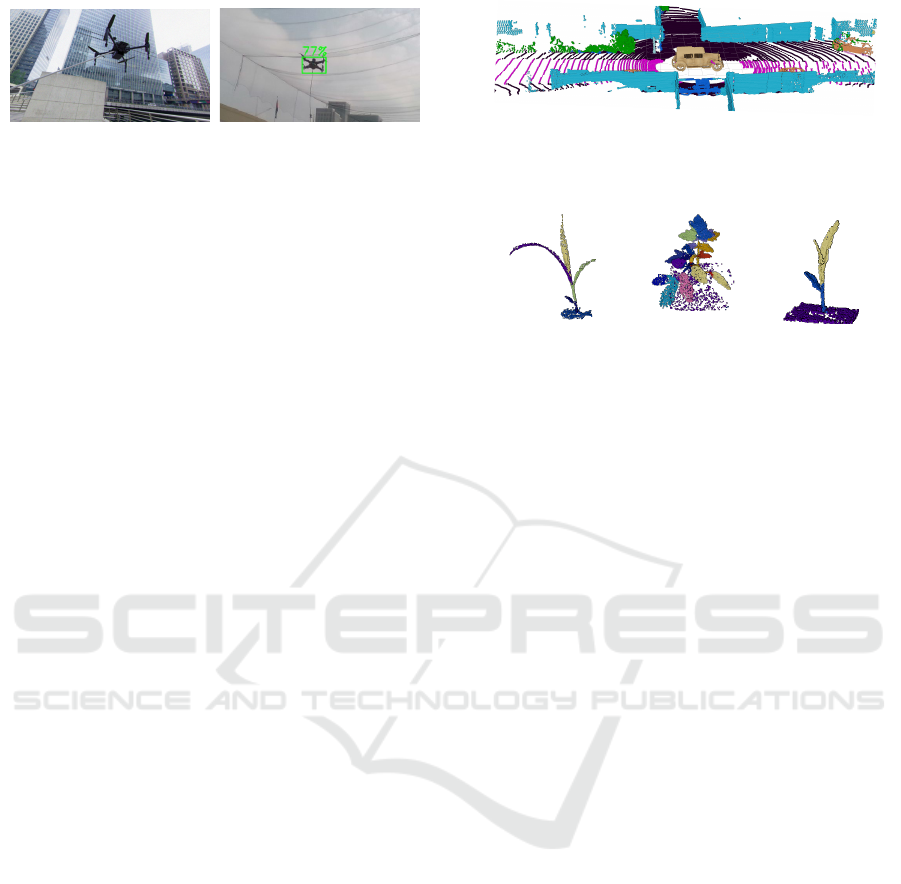
a) Synthetic DJI M100 drone b) Detection in real image

Figure 7: Synthetic data can be easily rendered and used

for deep learning applications. Images of drones together

with ground truth bounding box annotation were rendered

and used for training a drone detector.

8 APPLICATIONS

The ﬂexibility offered by EasyPBR allows it to be

used for a multitude of applications. We gather here a

set of real cases in which it was used.

8.1 Synthetic Data Generation

Deep learning approaches require large datasets in or-

der to perform supervised learning, and the effort in

annotating and labeling such datasets is signiﬁcant.

Consequently, interest has recently increased in using

synthetic data to train the models and thus avoid or

reduce the need for real labeled data.

EasyPBR has been used in the context of deep

learning to create realistic 2D images for object detec-

tion tasks. Speciﬁcally, it has been used for training a

drone detector capable of recognizing a drone in mid-

ﬂight. The model requires large amounts of data in

order to cope with the variations in lighting, environ-

ment conditions, and drone shape. EasyPBR was used

to create realistic environments in which we placed

various drone types that were rendered together with

ground truth bounding boxes annotations.

An example of a synthetic image and the output

from the drone detector model can be seen in Fig. 7.

The core of the Python code used to render the

synthetic images can be compactly expressed as:

view = Viewer()

view.load_environment_map("./map.hdr")

drone = Mesh("./drone.ply")

Scene.show(drone, "drone")

view.recorder.record("img.png")

8.2 Visualizer for 3D Deep Learning

Many recent 3D deep learning applications take as in-

put either raw point clouds or voxelized clouds. Visu-

ally inspecting the inputs and outputs of the network

is critical for training such models.

Figure 8: Point cloud segmented by LatticeNet (Rosu

et al., 2020) and visualized with the colormap of Se-

manticKITTI (Behley et al., 2019).

Figure 9: Instance segmentation of plant leaves using Lat-

ticeNet (Rosu et al., 2020).

EasyPBR interfaces with PyTorch (Paszke et al.,

2017) and allows for conversion between the CPU

data of the point cloud and GPU tensors for model

input and output. EasyPBR is used for data loading

by deﬁning a parallel thread that reads point cloud

data onto the CPU and then uploads to GPU tensors.

After the model processes the tensors, the prediction

is directly read by EasyPBR and used for visualiza-

tion. An example of 3D semantic segmentation and

instance segmentation of point clouds can be seen

in Fig. 8 and Fig. 9 where our tool was used for vi-

sualization and data loading.

Inside the training loop of a 3D deep learn-

ing approach, Python code similar to this one can

be used for visualization and input to the network:

cloud = Mesh("./lantern.obj")

points = eigen2tensor(cloud.V)

pred = net(points)

cloud.L = tensor2eigen(pred)

Scene.show(cloud, "cloud")

8.3 Animations

EasyPBR can also be used to create simple 2D and

3D animations. The 3D viewer keeps a timer, which

starts along with the creation of the application. At

any point, the user can query the delta time since the

last frame and perform incremental transformations

on the objects in the scene.

Additionally, the user can create small rigid kine-

matic chains by specifying a parent-child hierarchy

between the objects. Transformations of the parent

object will, therefore, also cause a transformation of

the child. This is useful when an object is part of an-

other one.

EasyPBR: A Lightweight Physically-based Renderer

251

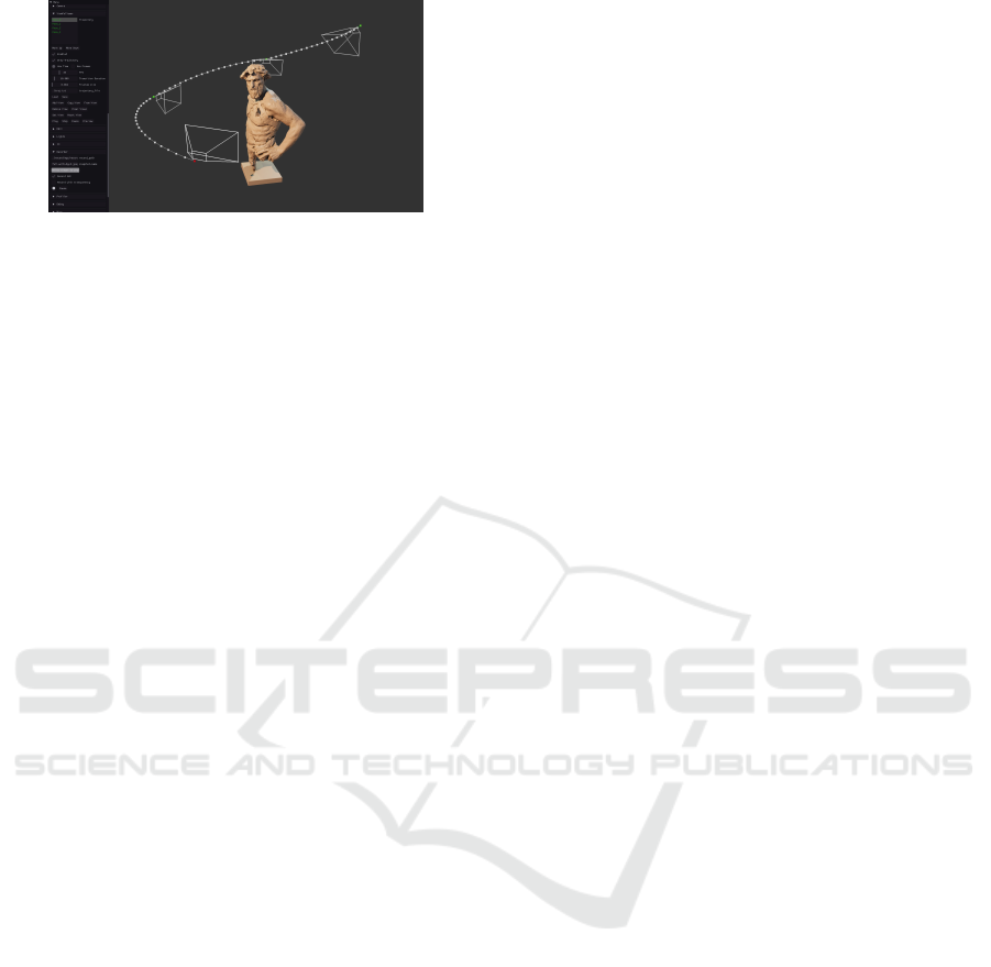
Figure 10: Viewer GUI and camera trajectory for recording

a video of the 3D object.

8.4 Recording

EasyPBR can be used both for taking screenshots of

the scene and for recording movies while the virtual

camera is moving through the environment. Through

the GUI, the user can place a series of key-poses

through which the camera should move. The user then

speciﬁes the time to transition from one pose to an-

other and lets the animation run. The camera linearly

interpolates between the speciﬁed SE(3) poses while

continuously recording. The images saved can then

be converted into a movie.

An example of the camera trajectory surrounding

an object to be captured can be seen in Fig. 10.

9 CONCLUSION

We presented EasyPBR, a physically-based renderer

with a focus on usability without compromising vi-

sual quality. Various state-of-the-art rendering meth-

ods were implemented and integrated into a frame-

work that allows easy conﬁguration. EasyPBR sim-

pliﬁes the rendering process by automatically choos-

ing parameters to render a speciﬁc scene, alleviating

the burden on the user side.

In future work, we intend to make EasyPBR eas-

ier to integrate for remote visualizations and also add

further effects like depth of ﬁeld and transparencies.

We make the code fully available together with the

scripts to create all the ﬁgures shown in this paper. We

hope that this tool will empower users to create visu-

ally appealing and realistic images without sacriﬁcing

performance or enforcing the burden of a steep learn-

ing curve.

REFERENCES

3D Scan Store (2020). 3D scan store. https://www.

3dscanstore.com/blog/Free-3D-Head-Model.

Bavoil, L. and Sainz, M. (2008). Screen space ambient oc-

clusion. http://developers.nvidia.com.

Behley, J., Garbade, M., Milioto, A., Quenzel, J., Behnke,

S., Stachniss, C., and Gall, J. (2019). SemanticKITTI:

A dataset for semantic scene understanding of lidar se-

quences. In IEEE International Conference on Com-

puter Vision (ICCV), pages 9297–9307.

Blender Online Community (2018). Blender - a 3D mod-

elling and rendering package. http://www.blender.org.

Boucheny, C. and Ribes, A. (2011). Eye-dome lighting: a

non-photorealistic shading technique. Kitware Source

Quarterly Magazine, 17.

Cignoni, P., Callieri, M., Corsini, M., Dellepiane, M.,

Ganovelli, F., and Ranzuglia, G. (2008). Meshlab:

an open-source mesh processing tool. In Eurograph-

ics Italian Chapter Conference, volume 2008, pages

129–136. Salerno.

Cook, R. L. and Torrance, K. E. (1982). A reﬂectance model

for computer graphics. ACM Transactions on Graph-

ics (ToG), 1(1):7–24.

Droeschel, D., Schwarz, M., and Behnke, S. (2017). Con-

tinuous mapping and localization for autonomous

navigation in rough terrain using a 3D laser scanner.

Robotics and Autonomous Systems, 88:104–115.

Epic Games (2007). Unreal Engine. https://www.

unrealengine.com.

Fdez-Ag

uera, C. J. (2019). A multiple-scattering microfacet

model for real-time image based lighting. Journal of

Computer Graphics Techniques (JCGT), 8(1):45–55.

Jacobson, A., Panozzo, D., et al. (2018). libigl: A simple

C++ geometry processing library. https://libigl.github.

io/.

Karis, B. (2013). Real shading in Unreal Engine 4. Proc.

Physically Based Shading Theory Practice.

Marmoset (2020). Marmoset toolbag. https://marmoset.co/

toolbag/.

Paszke, A., Gross, S., Chintala, S., Chanan, G., Yang, E.,

DeVito, Z., Lin, Z., Desmaison, A., Antiga, L., and

Lerer, A. (2017). Automatic differentiation in pytorch.

Reeves, W. T., Salesin, D. H., and Cook, R. L. (1987). Ren-

dering antialiased shadows with depth maps. In 14th

Annual Conference on Computer Graphics and Inter-

active Techniques, pages 283–291.

Reinhard, E., Stark, M., Shirley, P., and Ferwerda, J. (2002).

Photographic tone reproduction for digital images. In

29th Annual Conference on Computer Graphics and

Interactive Techniques, pages 267–276.

Rosu, R. A., Sch

utt, P., Quenzel, J., and Behnke, S. (2020).

Latticenet: Fast point cloud segmentation using per-

mutohedral lattices. In Proceedings of Robotics: Sci-

ence and Systems (RSS).

Schroeder, W. J., Avila, L. S., and Hoffman, W. (2000).

Visualizing with VTK: a tutorial. IEEE Computer

Graphics and Applications, 20(5):20–27.

uckler, J. and Behnke, S. (2014). Multi-resolution surfel

maps for efﬁcient dense 3D modeling and tracking.

Journal of Visual Communication and Image Repre-

sentation, 25(1):137–147.

Williams, L. (1978). Casting curved shadows on curved sur-

faces. In 5th Annual Conference on Computer Graph-

ics and Interactive Techniques, pages 270–274.

GRAPP 2021 - 16th International Conference on Computer Graphics Theory and Applications

252