
A Neural Network with Adversarial Loss for Light Field Synthesis from
a Single Image
∗
Simon Evain and Christine Guillemot
Inria, Rennes, France
Keywords:
Monocular, View Synthesis, Deep Learning, Light Field, Depth Estimation.
Abstract:
This paper describes a lightweight neural network architecture with an adversarial loss for generating a full
light field from one single image. The method is able to estimate disparity maps and automatically identify
occluded regions from one single image thanks to a disparity confidence map based on forward-backward
consistency checks. The disparity confidence map also controls the use of an adversarial loss for occlusion
handling. The approach outperforms reference methods when trained and tested on light field data. Besides,
we also designed the method so that it can efficiently generate a full light field from one single image, even
when trained only on stereo data. This allows us to generalize our approach for view synthesis to more diverse
data and semantics.
1 INTRODUCTION
View synthesis has been a very active field of research
in the computer vision and computer graphics com-
munities for many years ((Woodford et al., 2007),
(Horry et al., 1997)), and it has known significant ad-
vances thanks to the emergence of deep learning tech-
niques. In this paper, we tackle a specific case of this
problem: to synthesize an entire light field from one
single image. This problem has a variety of applica-
tions, such as generating several views of a scene, ex-
tracting depth and automatically identifying occluded
regions from images captured with regular 2D cam-
eras.
Working from one single image is a very challeng-
ing problem, for at test time, the approach lacks infor-
mation, e.g. on scene geometry. The method hence
needs strong priors on scene geometry and semantics.
Learning-based methods are therefore very good can-
didates for these tasks, since priors can be automat-
ically learnt from data. In this paper, we describe a
method that is able to produce an entire light field, es-
timate scene depth and identify occluded regions from
just one single image. This way, we can benefit from
light field features without requiring a light field cap-
ture set-up, e.g., simulating perspective shift and post-
capture digital re-focusing. We propose a lightweight
∗
This work has been funded by the EU H2020 Re-
search and Innovation Programme under grant agreement
No 694122 (ERC advanced grant CLIM).
architecture based on (Evain and Guillemot, 2020),
but enhanced to be able to generate an entire light field
and to better handle occlusions using an adversarial
approach. The network is trained on pairs of images
and learns to perform a forward and backward view
synthesis, with two independent branches, thanks to
the estimation of two disparity maps. Checking the
consistency of the two independent predictions allows
us to identify occluded regions and compute a dispar-
ity confidence map. At test time, the network only
needs one image to compute the two disparity maps
that are then used to identify the occluded regions.
This disparity confidence map is used to control the
application of an adversarial technique for occlusion
handling. We show that the network can be trained on
light field data, and that it outperforms reference tech-
niques trained on light field datasets, such as (Srini-
vasan et al., 2017), in terms of reconstructed light
field quality.
Now, training on light field data as in (Srinivasan
et al., 2017) necessarily restricts the scope of the ap-
proach, as this requires a large amount of data that
is not easy to capture. Besides, such monocular ap-
proaches are also bound a lot by semantics of the
training data, making it hard to train a network that
can be usable for a variety of scene geometry and se-
mantics, unless a sufficient number of examples of
diverse scenes is present in the training set. Exist-
ing light field datasets are in general too limited to
meet that requirement. We show that the proposed
Evain, S. and Guillemot, C.
A Neural Network with Adversarial Loss for Light Field Synthesis from a Single Image.
DOI: 10.5220/0010268701750184
In Proceedings of the 16th International Joint Conference on Computer Vision, Imaging and Computer Graphics Theory and Applications (VISIGRAPP 2021) - Volume 5: VISAPP, pages
175-184
ISBN: 978-989-758-488-6
Copyright
c
2021 by SCITEPRESS – Science and Technology Publications, Lda. All rights reserved
175

architecture can be trained on stereo content. This
drastically increases the amount of possible training
data that can be exploited by our approach. We show
that the proposed network produces very plausible
and good-quality light fields even when trained from
stereo images with large baselines as in the KITTI
dataset ((Geiger et al., 2012)), and this way produces
light fields with large fields of view. In summary, our
contributions are:
• A lightweight neural network based on (Evain and
Guillemot, 2020), extended to be able to generate
a full light field from one single view, with occlu-
sion handling relying on both a computed dispar-
ity confidence map and an adversarial approach.
• A light field synthesis method from one single
image that not only outperforms reference meth-
ods when trained and tested on light field data,
but that can also generalize to much more diverse
scenes, thanks to its ability to be trained on stereo
datasets. The method hence enables convincing
light field features (e.g., digital refocusing, virtual
camera motion) from only single 2D images.
1.1 Related Work
1.1.1 Monocular Stereo View Synthesis
Monocular view synthesis refers to the generation of
new views from one single image. This problem has
been tackled before the emergence of deep learning
techniques, however with some limitations, e.g. with
extremely similar images ((Woodford et al., 2007)), or
with scenes presenting very similar geometry ((Horry
et al., 1997)). Solving this difficult problem requires
strong scene priors, which can be efficiently learned
from data by using deep learning techniques.
The easiest set-up for monocular view synthesis
is the stereo case: given a pair of images, the aim is
to generate one image from the other. Usually, the
two cameras are kept in the same set-up, e.g. in terms
of relative distance between the cameras throughout
the training dataset, and the network implicitly learns
these set-up conditions. The pioneering work in the
domain is deep3D ((Xie et al., 2016)) with a network
designed to work on a dataset of 3D movies. The ap-
proach automatically generates a 3D sequence from a
2D sequence. A soft measure of disparity is estimated
from the input image and is used to warp the final
prediction. This method produces images of convinc-
ing quality. However, the network is bound to one
specific resolution, which implies training several net-
works for various resolutions. Besides, its number of
parameters is very high (around 60 million parame-
ters for a 512 × 256 resolution for the KITTI base-
line), and the network is not able to accurately process
occlusions. Finally, the produced images tend to be
blurry. Other approaches, such as (Evain and Guille-
mot, 2020), evolve over the concept by producing the
final image by merging a disparity-based warped pre-
diction and a prediction based on direct minimization.
Even if the approach outperforms state-of-the-art in
the stereo domain, its scope (stereo case only) is still
limited. The authors in (Ivan et al., 2019) also uti-
lize an appearance flow and spatio-angular consistent
loss functions and show that their model can produce
novel views of good quality in the case of densely
sampled light fields as those captured by Lytro Illum
cameras. Finally, we can also cite the approach in
(Shih et al., 2020) which converts a RGB-D input
image into a layered depth image (LDI) representa-
tion with explicit pixel connectivity. The authors then
use a learning-based inpainting model to synthesize
content in the occluded regions. While the addressed
problem has some similarities with ours, in particular
concerning occlusion handling, the authors assume a
RGB-D input image while we consider a simple RGB
input image.
1.1.2 Light Field View Synthesis
Light field imaging is based on the principles of in-
tegral imaging pioneered by Lippmann ((Lippmann,
1908)) in 1908. Due to technical challenges, it took
several decades before having practical light field
camera designs, e.g. with the work of (Ng, 2006).
Thanks to the ability to distinguish rays of light,
light field cameras permit a planar change of view-
point, as well as post-capture digital refocusing.
Given how complex a light field set-up can be (no-
tably in the case of camera arrays), and how memory-
consuming they are, view synthesis for light fields
soon became an important field of research to cope
with these issues. In (Kalantari et al., 2016), the au-
thors design a method to build a full light field from 4
corner images only. To do so, a cascade of two convo-
lutional neural networks (one for disparity and one for
color estimation) is employed, producing high-quality
images.
In (Mildenhall et al., 2019), an approach is pro-
posed based on the concept of Multi-Plane Image
(MPI) representation, first introduced in (Zhou et al.,
2018), to reconstruct a light field from a set of un-
structured image captures. The MPI representation is
a stack of parallel planes, regularly sampled in dispar-
ity, with a measure of visibility depending, for every
plane, on whether the pixel is at the foreground or the
background. The results are impressive but require
several input images (4 or 5) to be able to reconstruct
the light field. In contrast, our method only requires
VISAPP 2021 - 16th International Conference on Computer Vision Theory and Applications
176

one image to be able to generate light fields.
The authors in (Srinivasan et al., 2017) tackle the
issue of generating a full light field from one sin-
gle image. The approach takes the central view of
the light field as input, and seeks to generate the
light field by respecting the epipolar consistency con-
straint. The presented results are good quality, but
the overall approach comes with some limitations:
it obtains its more significant results on the Flowers
dataset, a dataset of images with very strong simi-
larities in scene semantics and geometry. When the
dataset gets a bit more complex and diverse, the ap-
proach encounters difficulties. Besides, working from
the epipolar constraint also means that the approach
gains from working with a large number of views
with small baselines at training time, which makes
the training process very long. More importantly, the
method requires a light field dataset that should be
large enough, and consistent enough in both seman-
tics and geometry. This kind of dataset is very rare,
and the method cannot be efficiently trained on other
data than light fields. In contrast, our method is able
to obtain very good results on the Flowers dataset, and
thanks to its ability to be trained on stereo content,
can also produce light fields with more generic and
diverse scenes.
Finally, the problem of light field view synthesis
from one single image has been recently addressed
in (Tucker and Snavely, 2020) where the authors first
construct a MPI representation from the input image,
and then warp this MPI to generate new light field
viewpoints. While this approach gives good results,
the network is quite heavy (around 47 million param-
eters).
1.1.3 Model-based View Synthesis
Methods have also been developed to tackle monoc-
ular view synthesis with the help of models or cam-
era set-up parameters. In (Sun et al., 2018), through
the blending of two predictions, a 6 Degrees of Free-
dom vector is obtained from input set-up parameters.
Even if the results are impressive for ranges of trans-
formation that have been learnt and processed during
training, when requiring a transformation which has
not been studied by the network, the method is usu-
ally much less efficient. To tackle the goal of gen-
erating a light field from stereo content, the method
is not adapted. Other methods ((Park et al., 2017),
(Tulsiani et al., 2018)) have been developed to gener-
ate new views by blending two predictions, including
one to be applied only in occluded regions. While
the method in (Park et al., 2017) is very efficient
on 3D models, or very simple scenes, it is less effi-
cient on natural images. Besides, it requires ground
truth occlusion maps in the training set, which are not
easy to capture. This reduces the amount of datasets
that can be used for training. The authors in (Tul-
siani et al., 2018) present a method able to distin-
guish the foreground from the background through
learning. Even if the results are interesting, they re-
quire a significantly heavier architecture than ours in
terms of number of parameters. In our case the oc-
cluded regions are automatically identified through
forward-backward checks, and we use an adversarial
loss to generate plausible content in occluded regions.
GANs ((Goodfellow et al., 2014)) have been shown
to be very useful for inpainting, e.g. in (Pathak et al.,
2016) where the unknown region is completed with a
mix of pixel-wise and adversarial-based predictions,
as well as for video generation (Clark et al., 2019).
Note that GANs have also been used in (Ruan et al.,
2018) to synthesize a light field from one single im-
age, however the problem is posed as a problem of
image super-resolution and the solution is therefore
based on image super-resolution approaches. In our
method, the use of the adversarial loss in the occluded
regions is controlled by an estimated disparity confi-
dence map. The authors in (Mildenhall et al., 2020)
address the problem of view synthesis by first regress-
ing from a continuous 5D representation of the scene
to a volumetric representation with volume densities
and view-dependent colors. This volumetric scene
function is then used together with volume rendering
techniques to generate novel light field views.
2 DESCRIPTION OF THE
METHOD
While the proposed method builds upon the architec-
ture in (Evain and Guillemot, 2020) designed for gen-
erating new views from one single image in a stereo
setting, it is extended here in order to be able to gener-
ate an entire light field from one single input view. In
addition, the network is designed in such a way that it
can be trained either with stereo content or using pairs
of light field views. While the network can be trained
from stereo content as well as from pairs of light field
views, when using classical stereo content to train the
network, the pipeline is adapted to account for natu-
rally missing information, e.g., related to scene geom-
etry, through the resort to the Refiner, as explained in
sections 2.3 and 2.5.
2.1 Disparity-Based Predictor (DBP)
The Disparity-Based Predictor (DBP) is a neural
network made up of two branches, accounting for
A Neural Network with Adversarial Loss for Light Field Synthesis from a Single Image
177
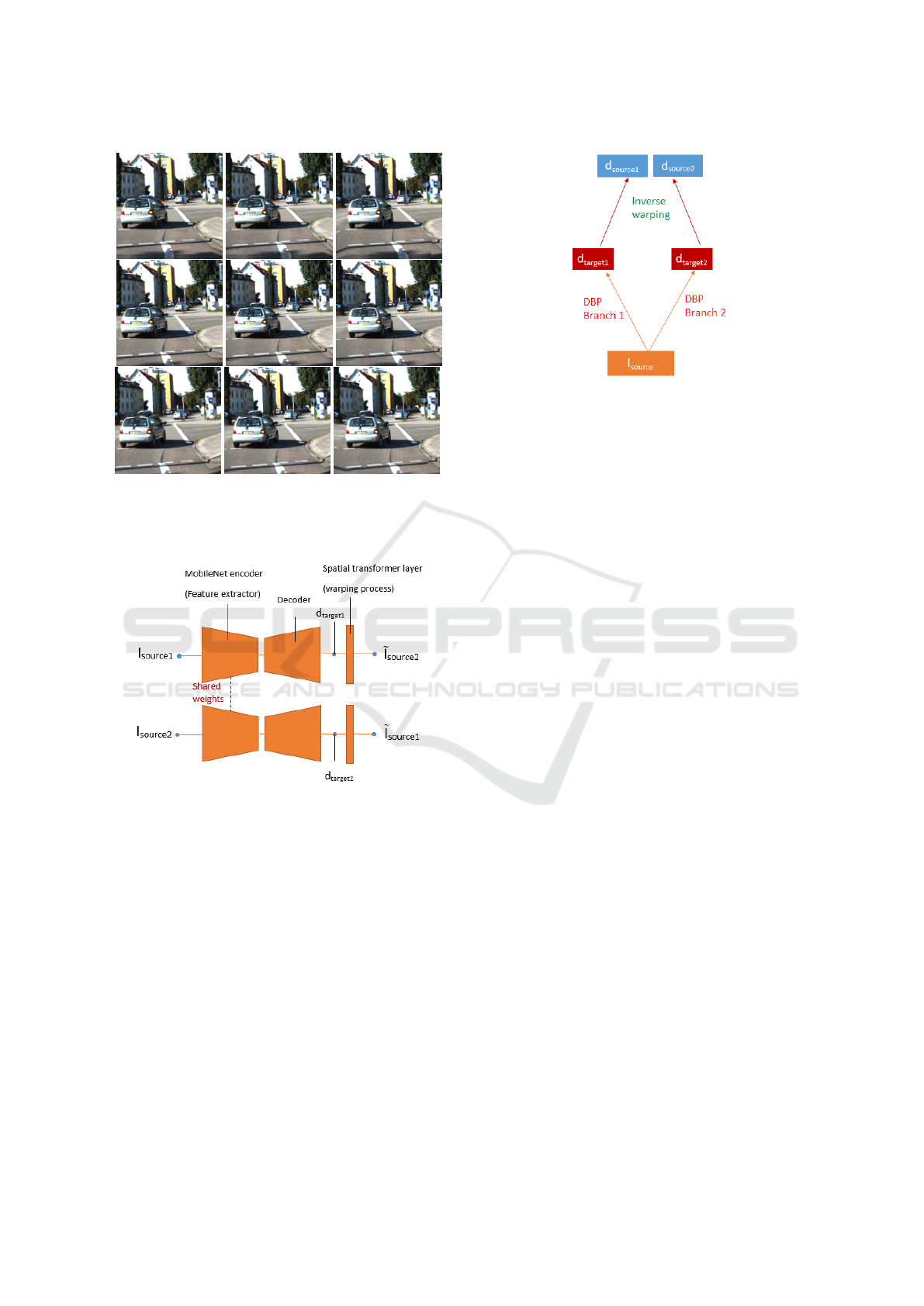
Figure 1: A light field generated from one single image
(input is the central view in the figure). The approach is
trained on KITTI stereo contents, and is augmented using
our method at test time to generate the light field.
Figure 2: Outline of the DBP section of our architecture.
both the Feature Extractor and the Decoder, as shown
in figure 2. It receives one single input image and
estimates a disparity map. Trained with a pair of
views, the two branches of the DBP take one image
of the pair as input, and consider the other image as
ground truth. In each branch, the Feature Extractor
is used to extract features of the input image, using
a MobileNet architecture, with weights shared with
the other branch. The weights are initialized with
ImageNet ((Deng et al., 2009)) weights. A second
part in each branch, the Decoder, produces a dispar-
ity map through upsampling layers and using skip-
connections. Finally, a spatial transformer layer is
used to warp the disparity map to predict a view.
This first prediction is based on the warping of pixels,
hence the result is usually sharp, but artifacts may re-
Figure 3: Diagram depicting the employed confidence
method.
main due to disparity errors, in particular in occluded
regions.
2.2 Estimating the Prediction
Confidence
The next step consists in identifying the regions not
well handled by DBP and the warping process. In
order to compute the confidence we have in our first
prediction, we use the already trained DBP, and we
follow the protocol defined in figure 3. We send as in-
put of our two branches the same input image I
source
.
This will give us two independent predictions in dis-
parity, centered on two different target views (d
target1
and d
target2
). We then re-warp these disparities back
onto the source view (giving us d
source1
and d
source2
),
and we take as confidence measure C
γ
their difference,
using the following expression:
C
γ
= exp(−γ|d
source1
− d
source2
|) (1)
We can note that in contrast with the method in
(Evain and Guillemot, 2020), the error is directly
computed and not estimated using a trained network.
Doing this simplifies the learning process, and allows
us to reduce the number of parameters (a network can
be removed when comparing with (Evain and Guille-
mot, 2020)). It is also a way to improve the confi-
dence map, so that occluded regions are better identi-
fied, as shown in the Results section.
2.3 Refiner based on a GAN
To correct errors in lower confidence regions, and to
account for the fact that the corresponding informa-
tion is not available at test time, we use a Refiner net-
work trained using an adversarial loss combined with
a pixel-wise metrics. This leads to plausible estimates
VISAPP 2021 - 16th International Conference on Computer Vision Theory and Applications
178

of the pixels in the occluded regions. The refiner net-
work is actually the generator of a Wasserstein GAN
((Arjovsky et al., 2017)), and adversarial learning is
carried out only in regions of low confidence.
The refiner is built as an encoder-decoder structure
with skip-connections. It is made up of a succession
of Spectrally Normalized convolutional layers (as first
described in (Miyato et al., 2018)). The discriminator
is also built using these layers. To make sure that the
learned distribution remains faithful to the input and
ground truth data, we also add pixelwise and gradient-
wise metrics besides the Wasserstein loss. This allows
us to fill occluded regions with synthesized contents,
which will be both realistic (thanks to the adversarial
loss) and as faithful as possible (thanks to the pixel-
wise metrics).
At test time, we only use the generator part of the
adversarial process to synthesize our view. It takes
as input the warped prediction, as well as the esti-
mated disparity map. The final predicted view V
f in
is obtained by combining the two predictions using
the confidence map as
V
f in
= C
γ
V
disp
+ (1 −C
γ
)V
re f
∗ (2)
where V
disp
is the output of DBP and an input to the
refiner, and V
re f
the output of the refiner, and C
γ
the
computed confidence map.
The method can be tailored to be efficiently
trained on both light fields and stereo content. There
is one refiner per branch, which is applied in both
learning and test time.
2.4 Training on Light Fields
When using light fields for training, we have access
to both horizontal and vertical disparities, hence the
DBP can be trained to estimate these two disparities
and produce the corresponding horizontal and vertical
warpings. We extract pairs of views by taking the cen-
ter view as one of the two images of the pair, and the
other one randomly within the light field. The max-
imum disparities of the light field are taken as refer-
ence. When working on views which are not extreme,
and assuming a regular sampling of views in struc-
tured light fields, we estimate the disparity d
int
of an
intermediate view by interpolation as
d
int
(x) = αd(x − (1 − α)d(x)) (3)
where α represents the targeted position, and x the
bidimensional coordinates. This allows us to obtain
an interpolated disparity map for warping, that will
tend to favor background disparity for occluded re-
gions, and lead to more plausible results than when
simply multiplying the disparity map.
2.5 Training on Stereo Content
The method can also be trained on stereo data, and be
used to generate full light fields. In this case, we can
only train the method with horizontal disparity, and
have to infer vertical disparity at test time. We there-
fore add a simple module to infer the vertical disparity
at test time, once the network was trained on stereo
contents. The new, two-channel disparity map d
new
is obtained from the horizontal, predicted one, by ap-
plying the following transformation to the horizontal
disparity map d
hor
:
d
new
(y, x ) = αd
hor
(α
y
d
hor
(x), x − (1 −α
x
)d
hor
(x)))
(4)
where y accounts for vertical coordinates, while x ac-
counts for horizontal coordinates, and α = (α
y
, α
x
) is
a set of parameters accounting for the relative posi-
tion of the requested view relatively to the input view.
Given that the warped disparity map may however
contain errors especially in the foreground near the
borders of the image, we improve it by applying an
auto-regressive extrapolation along the vertical lines
and from the 50 previous points. The rest of the net-
work proceeds with the warped prediction, and refines
and automatically improves the occluded regions at
test time.
2.6 Summary
In summary, the procedure is as follows:
• From a pair of images, learning the disparity and
warping from it through the DBP to generate one
from the other.
• Through a confidence computation obtained by
inputting the same image in both branches, deter-
mining which regions are likely to be accurate.
• In the regions with low-confidence, using a refiner
with adversarial learning to improve the results.
3 LEARNING PROCEDURE
Let L
DBP
and R
DBP
be the DBP-based predictions, and
L and R the ground truth images, and d
L
and d
R
the
disparity maps for the warping towards predictions L
and R. We first train the DBP using the metrics:
λ
0
(||L
DBP
− L||
1
+ ||R
DBP
− R||
1
)
+ λ
1
(||∇L
DBP
− ∇L||
1
+ ||∇R
DBP
− ∇R||
1
)
(5)
Before training the Refiner, we add a step of geomet-
rical restructuring for the DBP. Finally, we freeze the
A Neural Network with Adversarial Loss for Light Field Synthesis from a Single Image
179

weights of DBP, and train the Refiner in order to min-
imize the loss function
λ
4
(||L
REF
− L||
1
) + λ
5
(||∇L
REF
− ∇L||
1
)
+ λ
6
(||L
∗
− L||
1
) + λ
7
(||∇L
∗
− ∇L||
1
+ λ
8
L (L
∗
, L)
(6)
where L
REF
is the prediction performed by the Re-
finer, L the ground truth image, L
∗
the final combined
prediction L
∗
= C
γ
L
DBP
+ (1 − C
γ
)L
REF
, and L the
Wasserstein loss. The discriminator for the adversar-
ial process is trained using only this Wasserstein loss.
For the hyperparameters, we consider: γ = 0.08, λ
0
=
0.80, λ
1
= 0.20, λ
4
= 0.27, λ
5
= 0.054, λ
6
= 0.54,
λ
7
= 0.135, λ
8
= 0.01. We optimize our approach us-
ing the Adam algorithm ((Kingma and Lei Ba, 2015)),
with β
1
= 0.9 and β
2
= 0.999. We use a learning
rate of 0.0001 for the overall network (with 0.00001
for the discriminator during training). The work was
implemented using TensorFlow ((Abadi et al., 2015))
and Keras ((Chollet et al., 2015)). The network was
stopped when no improvement in the validation met-
rics was obtained after 20 epochs. The network is
fully trained after only a few hours, and contains
around 6 million parameters at training time.
For the following experiments, our method for
training took as input patches of resolution 256 ∗ 256
(for the stereo case) or 256 ∗ 512 (for the light field
case), normalized between -1 and 1, with data aug-
mentation in 20 % of the cases, with random gamma
and brightness transformations. In this article, we
used two datasets for comparison: Flowers ((Srini-
vasan et al., 2017)) and KITTI ((Geiger et al., 2012)).
Flowers is a light field dataset, with rather small base-
lines, comprising around 3,000 light fields of flowers
in similar geometrical configurations. We systemati-
cally pick the central view as one element of the pair,
and we randomly choose another view as the other el-
ement of the pair. We adjust the value of α to account
for the coordinate of the selected view. As a start-
ing point, we only focus on one corner view as target
that we arbitrarily choose as the reference disparity
(α = (1, 1)). After 10 epochs, we add the rest of the
views as possible target views and the interpolation
process described in section 2.4 is then applied. We
perform a train-test-validation split, to be able to com-
pare our approach. KITTI is a stereo dataset which
depicts urban scenes, and contain pairs of images with
a very significant disparity gap between them. In this
work, we use 400 pairs of images randomly chosen as
training elements.
Table 1: Statistical comparisons between our method
trained on light field data (Ours), reference method LF4D
((Srinivasan et al., 2017)), and our stereo-based method
(Stereo). We display the mean PSNRs and SSIM on the
4 corner views (the most difficult ones to predict), as well
as on the full light field.
PSNR/SSIM Ours LF4D Stereo
4 corners 34.97/0.94 31.61/0.89 33.54/0.93
Full LF 38.41/0.96 35.10/0.94 37.16/0.95
4 EVALUATION
We compare the proposed approach to several meth-
ods: LF4D ((Srinivasan et al., 2017)), a method able
to predict a full light field from one single image,
by enforcing epipolar constraints within the predicted
light field, using the code provided by the authors. We
also compare visually our approach with the method
in (Sun et al., 2018), in the stereo case, using the net-
work provided by the authors. We also compare our
method to the recently published method (Evain and
Guillemot, 2020), and with the reference method (Xie
et al., 2016), both focused on working in a stereo set-
ting. To evaluate our stereo-based approach, we also
use it on Flowers by only training it from 2 aligned
views on the central line of the light field ((Srinivasan
et al., 2017)). For evaluation, we use PSNR, SSIM
and LPIPS ((Zhang et al., 2018)) as reference metrics.
Due to the visual nature of the task, we strongly rec-
ommend the reader to take a look at the Supplemen-
tary video, which displays other examples of views
synthesized using the proposed method.
4.1 Light Field View Synthesis Results
Training and Testing with Light Field Data. We
first focus on training and testing the network with
light fields. For that, we use the Flowers dataset
((Srinivasan et al., 2017)). We evaluate predicted
views in comparison with the reference method LF4D
((Srinivasan et al., 2017)), by applying an identical
experimental protocol, in figures 4, 5 and 6, in table
1, as well as in the supplementary video. We see that
our approach clearly outperforms LF4D, both metric-
wise and visually.
We also use the Flowers dataset to evaluate our
stereo-training based approach, i.e. by only training
the network on stereo aligned pairs (extreme left-side
view - center view and center view - extreme right-
side view). The results (the last row of figure 4 and
table 1) show that our method, even when trained
on stereo content, manages to outperform the LF4D
monocular light field synthesis method, and is able to
produce high-quality light fields. This shows that our
VISAPP 2021 - 16th International Conference on Computer Vision Theory and Applications
180
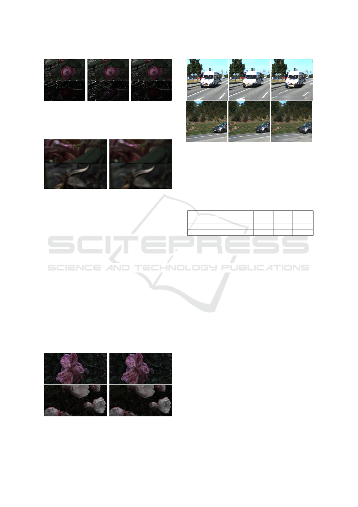
Figure 4: Visual prediction for a top-left image from the
Flowers test set, as well as the corresponding L1 errors, for,
from left to right, our method, LF4D ((Srinivasan et al.,
2017)) and the stereo version of our method. The errors
were multiplied with a factor of 3 for better visualization.
Figure 5: Close-up views from figure 4. On the left side,
our results, on the right side, the results obtained in (Srini-
vasan et al., 2017). We note that our results are sharper and
structurally more consistent.
stereo to light fields adaptation module is very effi-
cient.
Training on Stereo Content. We also train the net-
work using the stereo KITTI dataset ((Geiger et al.,
2012)), in order to build a full light field. The views
produced have no ground truth equivalent; only visual
evaluation is possible in this case. Visual results are
shown in figure 1 and in the supplementary video. To
evaluate our approach, we compare it visually to the
monocular part of the method in (Sun et al., 2018).
The network, also trained on KITTI, receives as in-
put one image and a transformation vector expressing
the relative coordinates of the target view. We spec-
ify to the pre-trained network a transformation vector
similar to ours.
We note that our approach clearly performs better
visually on this data (see figure 7). This is probably
Figure 6: Supplementary visual comparisons between our
work (left-side) and (Srinivasan et al., 2017) (right-side).
We note that our images are sharper and better quality.
Figure 7: Visual comparison of two of our predictions
with Sun’s method, for similar geometrical transformations
(from left to right, 2 sequences of: input, our prediction, and
the prediction obtained from (Sun et al., 2018)). The views
we produce are less blurry and have fewer distortions.
Table 2: Comparison of the results of our approach with 2
reference methods ((Evain and Guillemot, 2020), (Xie et al.,
2016)) in a stereo setting. For PSNR and SSIM, the higher,
the better. For LPIPS, the lower, the better.
KITTI Test Set PSNR SSIM LPIPS
Ours 19.96 0.76 0.130
(Evain and Guillemot, 2020) 19.24 0.74 0.139
Deep3D ((Xie et al., 2016)) 19.08 0.74 0.220
because the vertical transformations are not present
in the KITTI training set, and can thus not be learnt
efficiently by the method in (Sun et al., 2018). Given
that our approach is optimized to generate the light
field, we are able for this task to obtain more realistic
results.
To evaluate metric-wise our predictions, we also
compare them with stereo-based view synthesis meth-
ods (Evain and Guillemot, 2020) and (Xie et al.,
2016) in table 2, on the KITTI test set, in a stereo
setting. We note that our approach significantly out-
performs these two reference methods in the 3 chosen
metrics. We can note that we obtain those results with
a smaller number of parameters (notably, (Evain and
Guillemot, 2020) has 200,000 more parameters). We
show in figure 8 a visual stereo prediction, associated
with the L1 error. We can see that the predicted view
is rather high-quality.
Finally, we compare our confidence computation
process with the one described in (Evain and Guille-
mot, 2020) in figure 9. We note that our occlusion
identification process is significantly more efficient.
Testing on Natural Images. We can also test our
network on natural images, captured using a smart-
phone. It allows us to produce a full light field from
one single image. A visual example of it is shown in
figure 10.
A Neural Network with Adversarial Loss for Light Field Synthesis from a Single Image
181
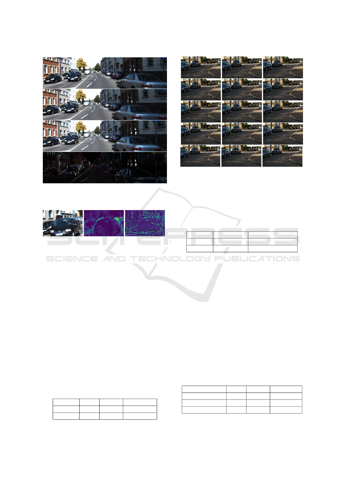
Figure 8: Result of our approach in a stereo setting, on the
KITTI test set, for evaluation. From top to bottom: input
image, our prediction, ground truth image, L1 error.
Figure 9: Visual evaluation and comparison of the confi-
dence map. Yellow means low-confidence. From left to
right: our prediction, confidence map returned by our ap-
proach, confidence map returned by (Evain and Guillemot,
2020) in the same setting. We note that our way to compute
the confidence map is significantly better at specifically cap-
turing occluded regions.
4.2 Ablation Study
Impact of the Confidence-based Refiner. We eval-
uate the impact of the refiner on the result in tables
3 and 5. We can note that it significantly increases
the performance both in PSNR and SSIM for both
datasets. Its contribution is, though, more significant
when working on KITTI, due to its more significant
occluded regions. We also evaluate its positive contri-
bution when training the approach on stereo contents,
and using it to generate light fields in table 4. We note
that the Refiner in this case also allows to significantly
improve the performance of the approach.
Table 3: Statistical comparisons for the ablation study on
the Flowers test set. No Refiner only uses the warped pre-
diction, No AL does not use adversarial learning.
Flowers Ours No AL No Refiner
PSNR 38.41 38.40 37.59
SSIM 0.96 0.96 0.95
Figure 10: A light field generated from one single image
(input is the central view in the figure). The approach is
tested on a natural image, captured using a smartphone. For
a result with higher resolution, we advise the reader to check
the supplementary video.
Table 4: Statistical comparisons for the ablation study on
the Flowers test set. Stereo ours is our stereo-based light
field synthesis method, Stereo No Refiner evaluates the pre-
diction when no refiner is used.
Flowers Stereo ours Stereo No refiner
PSNR 37.16 36.02
SSIM 0.95 0.93
Impact of Adversarial Learning. We also evalu-
ate the impact of our adversarial process on the re-
sult. We note that depending on the chosen dataset,
we do not draw the same conclusions. When working
on Flowers (see table 3), we note that the adversarial
process does not really have a significant impact. The
occluded regions in Flowers are indeed smaller and
then easier to fill, reducing the usefulness of the ad-
versarial loss.
On the other hand, when working on KITTI, we
can see that the adversarial process is much more ben-
eficial, giving an overall increase in PSNR and SSIM,
but more importantly a significantly better LPIPS
((Zhang et al., 2018)), showing that it is an adequate
way to improve the perceptiveness of our images. A
Table 5: Statistical comparisons for the ablation study on
the KITTI test set. No Refiner only uses the warped predic-
tion, No AL does not use adversarial learning.
KITTI Test Set Ours No AL No refiner
PSNR 19.96 19.85 18.87
SSIM 0.76 0.75 0.74
LPIPS 0.130 0.135 0.144
VISAPP 2021 - 16th International Conference on Computer Vision Theory and Applications
182
visual example of such an improvement on KITTI is
displayed in figure 11.
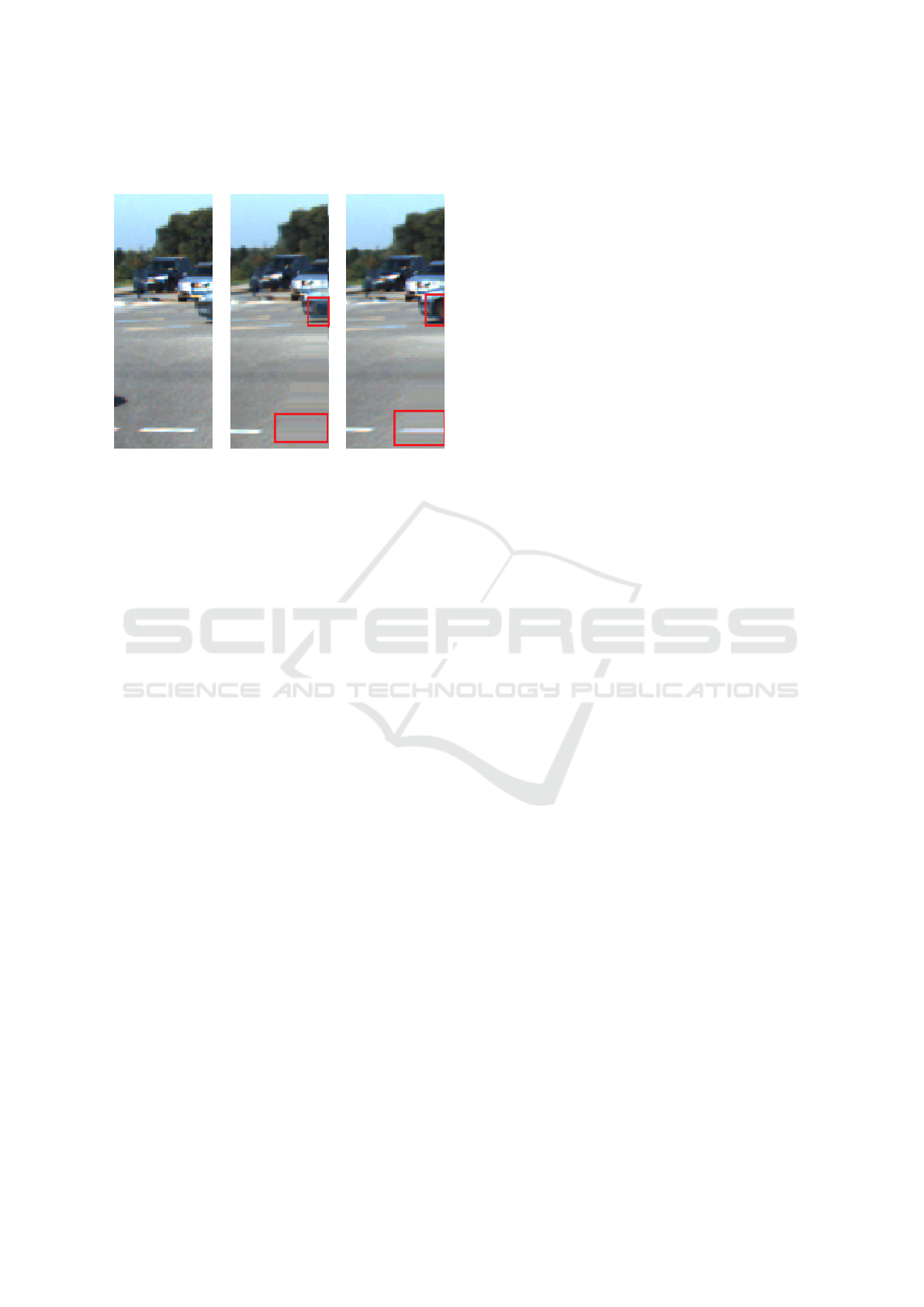
Figure 11: Contribution of adversarial learning. From left
to right, input image, prediction without adversarial learn-
ing, prediction with adversarial learning. We note that the
approach with adversarial learning is able to fill in these oc-
cluded regions more realistically (highlighted in red).
5 CONCLUSION
In this article, we have described a method able to
produce light fields, with a training from both light
field datasets and stereo datasets. The proposed
method allows us to generate high-quality light fields,
from only one single input image and for diverse im-
ages and semantics. We manage to achieve good per-
formance for producing these light fields, and are able
to use stereo data to produce light fields with a wider
variety of contents and semantics.
REFERENCES
Abadi, M., Agarwal, A., Barham, P., Brevdo, E., Chen, Z.,
Citro, C., Corrado, G. S., Davis, A., Dean, J., Devin,
M., Ghemawat, S., Goodfellow, I., Harp, A., Irving,
G., Isard, M., Jia, Y., Jozefowicz, R., Kaiser, L., Kud-
lur, M., Levenberg, J., Man
´
e, D., Monga, R., Moore,
S., Murray, D., Olah, C., Schuster, M., Shlens, J.,
Steiner, B., Sutskever, I., Talwar, K., Tucker, P., Van-
houcke, V., Vasudevan, V., Vi
´
egas, F., Vinyals, O.,
Warden, P., Wattenberg, M., Wicke, M., Yu, Y., and
Zheng, X. (2015). TensorFlow: Large-scale machine
learning on heterogeneous systems. Software avail-
able from tensorflow.org.
Arjovsky, M., Chintala, S., and Bottou, L. (2017). Wasser-
stein gans. ICML.
Chollet, F. et al. (2015). Keras. https://keras.io.
Clark, A., Donahue, J., and K., S. (2019). Adversarial video
generation on complex datasets.
Deng, J., Dong, W., Socher, R., Li, L., Li, K., and Fei-Fei,
L. (2009). Imagenet: A large-scale hierarchical image
database. CVPR.
Evain, S. and Guillemot, C. (2020). A lightweight neural
network for monocular view generation with occlu-
sion handling. PAMI.
Geiger, A., Lenz, P., and Urtasun, R. (2012). Are we ready
for autonomous driving? the kitti vision benchmark
suite. CVPR.
Goodfellow, I., Pouget-Abadie, J., Mirza, M., Xu, B.,
Warde-Farley, D., Ozair, S., Courville, A., and Ben-
gio, Y. (2014). Generative adversarial networks.
NIPS.
Horry, Y., Anjyo, K., and Arai, K. (1997). Tour into the
picture: using a spidery mesh interface to make ani-
mation from a single image. Proceedings of the 24th
annual conference on Computer graphics and inter-
active techniques, pages 225–232.
Ivan, A., Williem, and Park, I. K. (2019). Synthesizing a
4d spatio-angular consistent light field from a single
image.
Kalantari, N., Wang, T., and Ramamoorthi, R. (2016).
Learning-based view synthesis for light field cameras.
SIGASIA.
Kingma, D. and Lei Ba, J. (2015). Adam: a method for
stochastic optimization. ICLR.
Lippmann, G. (1908). La photographie int
´
egrale. Comptes-
Rendus de l’Acad
´
emie des Sciences.
Mildenhall, B., Srinivasan, P., Ortiz-Cayon, R., Kalantari,
N., Ramamoorthi, R., Ng, R., and Kar, A. (2019). Lo-
cal light field fusion: Practical view synthesis with
prescriptive sampling guidelines. ACM Transactions
on Graphics.
Mildenhall, B., Srinivasan, P. P., Tancik, M., Barron, J. T.,
Ramamoorthi, R., and Ng, R. (2020). Nerf: Repre-
senting scenes as neural radiance fields for view syn-
thesis.
Miyato, T., Kataoka, T., Koyama, M., and Yoshida, Y.
(2018). Spectral normalization for generative adver-
sarial networks. ICPR.
Ng, R. (2006). Digital light field photography.
Park, E., Yang, J., Yumer, E., Ceylan, D., and Berg, A.
(2017). Transformation-grounded image generation
network for novel 3d view synthesis. CVPR.
Pathak, D., Kr
¨
ahenb
¨
uhl, P., Donahue, J., Darrell, T., and
Efros, A. (2016). Context encoders: Feature learning
by inpainting. CVPR.
Ruan, L., Chen, B., and Lam, M. L. (2018). Light field
synthesis from a single image using improved wasser-
stein generative adversarial network. In Jain, E. and
Kosinka, J., editors, EG 2018 - Posters. The Euro-
graphics Association.
Shih, M.-L., Su, S.-Y., Kopf, J., and Huang, J.-B. (2020).
3d photography using context-aware layered depth in-
painting. In IEEE Conference on Computer Vision and
Pattern Recognition (CVPR).
Srinivasan, P., Wang, T., Sreelal, A., Ramamoorthi, R., and
Ng, R. (2017). Learning to synthesize a 4d rgbd light
field from a single image. ICCV.
A Neural Network with Adversarial Loss for Light Field Synthesis from a Single Image
183

Sun, S., Huh, M., Liao, Y., Zhang, N., and Lim, J. (2018).
Multi-view to novel view: Synthesizing novel views
with self-learned confidence. ECCV.
Tucker, R. and Snavely, N. (2020). Single-view view syn-
thesis with multiplane images. In The IEEE Con-
ference on Computer Vision and Pattern Recognition
(CVPR).
Tulsiani, S., Tucker, R., and Snavely, N. (2018). Layer-
structured 3d scene inference via view synthesis.
ECCV.
Woodford, O., Reid, I., Torr, P., and Fitzgibbon, A.
(2007). On new view synthesis using multiview
stereo. BMVC, pages 1–10.
Xie, J., Girshick, R., and Farhadi, A. (2016). Deep3d: Fully
automatic 2d-to-3d video conversion with deep convo-
lutional neural networks. ECCV.
Zhang, R., Isola, P., Efros, A., Shechtman, E., and Wang, O.
(2018). The unreasonable effectiveness of deep fea-
tures as perceptual metric. CVPR.
Zhou, T., Tucker, R., Flynn, J., Fyffe, G., and Snavely, N.
(2018). Stereo magnification: Learning view synthe-
sis using multiplane images. SIGGRAPH.
VISAPP 2021 - 16th International Conference on Computer Vision Theory and Applications
184
