Congestion-Aware Stochastic Path Planning and Its Applications in Real

World Navigation

Kamilia Ahmadi and Vicki H. Allan

Computer Science Department, Utah State University, Logan, Utah, U.S.A.

Keywords:

Stochastic Path Planning, Multi-Agent Systems, Congestion-Aware Modelling, Non-Linear Objective, Route

Planning under Uncertainty.

Abstract:

In the realm of path planning, algorithms use edge weights in order to select the best path from an origin point

to a speciﬁc target. This research focuses on the case where the edge weights are not ﬁxed. Depending on the

time of day/week, edge weights may change due to the congestion through the network. The best path is the

path with minimum expected cost. The interpretation of best path depends on the point of view of car drivers.

We model two different goals: 1) drivers who look for the path with the highest probability of reaching the

destination before the deadline and 2) the drivers who look for the best time slot to leave in order to have a

smallest travel time while they meet the deadline. Both of the goals are modelled based on the cost of the

path which is highly dependent on the level of congestion in the network. Minimizing the paths’ cost helps in

reducing trafﬁc in the city, alleviates air pollution, and reduces fuel consumption. Findings show that using our

proposed intelligent path planning algorithm which satisﬁes users’ goals and picks the least congested path is

more cost efﬁcient than picking the shortest-length path. Also, we show how agents’ goals and selection of

cost function impacts paths’ choice.

1 INTRODUCTION

Path planning ﬁnds a path from a speciﬁc origin to

a destination over a network of road segments. Path

planning algorithms use the road segment costs in or-

der to come up with the best path. If the road seg-

ments’ costs are ﬁxed, planning the best path through

the network is a well understood task via the algo-

rithms like Dijkstra and A* algorithms (Dijkstra and

W., 1959; Hart et al., 1968). However, in real world

navigation problems, depending on the level of con-

gestion on the road segments, the cost associated with

the legs of the trip changes over time. Also, it is not

feasible to use an adaptive algorithm in every step

due to the urgency in having a quick response to the

queries and hesitancy of drivers to change their route

frequently.

In modeling a city scale graph, congestion

changes throughout the day which results in having

uncertain costs on the road segments (Nikolova and

Karger, 2008; Rus, 2020; Geisberger et al., 2010;

Yaoxin Wu et al., 2016). Congestion is highly af-

fected by the path selection of drivers in the network.

In addition, there are many factors that affect the

congestion pattern such as road conditions, drivers’

path choice, time of the day, weather conditions, and

events throughout the city (Rus, 2020; Geisberger

et al., 2010; Wilkie et al., 2011; Sigal et al., 1980; Pi

and Qian, 2017; Niknami and Samaranayake, 2016).

We consider expected travel time on the road seg-

ments as the cost of that segment. The variabil-

ity of congestion level on road segments makes it a

stochastic network. Minimizing the paths costs, ul-

timately results in reducing the city scale congestion

by picking less congested paths. Reducing conges-

tion throughout the city has the beneﬁts of decreased

pollution, fewer accidents, less wasted time, and less

fuel costs (Chiabaut et al., 2009; Fan et al., 2005; Rus,

2020; Pi and Qian, 2017; Yaoxin Wu et al., 2016).

This paper focuses on path planning over a

stochastic network which is a graph of a city. The

challenge is to ﬁnd the best paths under uncertainty

and the constraints of real world domain. Agents are

car drivers which can pursue different goals: ﬁrst, the

ones who are not willing to take risk and look for the

path with highest probability of reaching destination

before a desired arrival time, even if it may take them

longer. Second, the agents who are open to take a

riskier decision if it helps them in having the small-

est en-route time. These agents are ﬂexible in leaving

Ahmadi, K. and Allan, V.

Congestion-Aware Stochastic Path Planning and Its Applications in Real World Navigation.

DOI: 10.5220/0010267009470956

In Proceedings of the 13th International Conference on Agents and Artiﬁcial Intelligence (ICAART 2021) - Volume 2, pages 947-956

ISBN: 978-989-758-484-8

947

anytime while they still need to make the trip.

To make it clearer, one good example of these kind

of agents’ goals is in the context of a package de-

livery system. For example, suppose that we guar-

antee the delivery of a package by 4 PM, otherwise

the customer doesn’t accept the delivery and we lose

the shipping costs. In that case, we are interested in

picking a path that has the highest chance of reach-

ing destination before the deadline to avoid losing the

shipping cost. The other possible case is delivering

perishable products. For example, if we promised the

delivery of perishable products before 6 PM to the

customers, we are interested to pick a path that has

the smallest en-route time due to the nature of our

package. In this case, we are ﬂexible in leaving any-

time, but we do need to have the smallest en-route

path while still making the destination before 6 PM.

As mentioned earlier, the deﬁnition of best path

differs based on the goal of the agents. For ﬁnding the

best path, queries have an origin, a destination and the

desired arrival time (deadline) along with the agents’

goals. Our proposed path planning framework, mod-

els the city as a stochastic network, utilizes pruning

techniques to reduce the size of search space, deﬁnes

the path costs, aligns them with agents goals and picks

the minimum cost path.

2 LITERATURE REVIEW AND

CONTRIBUTION

Miller-Hooks and Mahmassani (Miller-Hooks and

Mahmassani, 2000) consider travel costs as edge

weights of a navigation graph in their model. Costs

depend on travel times, and their goal is to ﬁnd the

least expected travel time in peak and non-peak time

of the day. Then they solve an equivalent determinis-

tic problem. The main concern with this framework is

there has been little work on considering uncertainty,

congestion awareness and time dependency of edge

weights in ﬁnding the optimal path.

Fan, Kalaba and Moore (Fan et al., 2005) consider

a special monotone increasing cost based on the prob-

ability of arriving late and suggests that the Gamma

distribution is natural for modelling stochastic edge

travel times. The probability calculation requires

computing a continuous-time convolution product.

Therefore, it makes the path planning a computation-

ally expensive and time consuming task.

Niknami et al (Niknami and Samaranayake,

2016), present a model to compute the route that max-

imizes the probability of on-time arrival in stochas-

tic networks. Their method uses a heuristic for the

optimal path that chooses the direction at every in-

tersection based on the current state by evaluating

zero-delay convolution on the path probability and ex-

pected travel time. However, they assume that travel

time distributions are exogenous (not impacted by in-

dividuals routing choices) which makes it not desir-

able as in realistic domain path choices are affected

by other drivers’ decisions as a major source of con-

gestion on stochastic networks.

Zhiguang (Cao, 2017), proposed the Probability

Tail model based on a cardinality minimization prob-

lem by directly utilizing travel time data on each

road link. Then, the minimization problem is ap-

proximately solved via relaxing the cardinality by

L1-norm, and formulating it as a mixed integer lin-

ear programming problem. For extracting the edge

weights, it uses travel time samples on each arc as in-

put and adopts some random distributions to generate

the weights. As the result, this model doesn’t consider

trafﬁc patterns for different times of a day.

Rus et al. (Rus, 2020) proposes stochastic path

planning method where edge weights are represented

as linear combination of mean and variance of travel

time (mean+ λ * variance) controlled by a λ parame-

ter. In their model, the key property is that the optimal

path occurs among the extreme points of the convex

hull containing all the path points. Then λ is used

to prune the search regions and selects only a small

number of λ values. The best path is found by Di-

jkstra (Dijkstra and W., 1959) based on minimizing

the cost function of two modelled goals: a) probabil-

ity tail model and b) mean risk model. Since, Rus’s

model uses exhaustive enumeration for path selection,

it’s run time in average is O(n

log

(n)).

In our work, we propose a path planning model

which uses Rus’s work (Rus, 2020) as a conceptual

framework but provides practical improvements on

top of it. Firstly, we do not linearly combine mean

and variance of travel time on edge weights. We con-

sider travel costs in intervals of 10 minutes for each

day of a week and extract the typical mean and vari-

ance on that edge for the speciﬁc time slots. Means

and variances are as short as 10 minutes time seg-

ments to present the variation in any given point of

day/time accurately. Also, we study three options of

cost functions (linear, exponential, and step cost func-

tion) to have a better understanding of main classes

of cost modelling and their impact in path selection.

However, the model is general enough to include any

cost function. (details of cost functions are explained

in 3.5)

Our proposed path planning algorithm has two

main steps: a) pruning search region to select few can-

didate paths among all possible paths, and b) Planning

an optimal path from the candidate paths in step a. In

ICAART 2021 - 13th International Conference on Agents and Artiﬁcial Intelligence

948

pruning phase, a node is expanded if expected mean

of the travel time of the approximate path through the

node is less then the user’s deadline. Proposed prun-

ing algorithm utilizes graph clustering and approxi-

mation techniques (explained in detail in 3.4). Major-

ity of pruning work utilizes pre-computation, which

makes it very efﬁcient and practical to real work do-

main. The second part of proposed path planning al-

gorithm focuses on picking the path which has the

minimum cost aligned with agents’ goals.

The last contribution of this paper focuses on

modelling agents’ goals. First group of agents are

looking for the path that maximizes the probability

of reaching a destination before the deadline (highest

probability path). Second group, look for the best de-

parture time slot in order to have the least travel time

and arrive at the destination before deadline, these

agents are interested to take riskier decision if it pro-

vides them shortest en-route time. Details of agents’

goal modelling is discussed in 3.6.

3 MODEL DESCRIPTION

3.1 Open Street Map Data

For building the city graph, we used Open Street Map

data (Haklay and Weber, 2008). Open Street Map is a

collaborative open source project which creates a free

editable map that can be used widely. Open Street

Map represents physical entities on the ground like

buildings, roads, intersections, bridges and so on. It

uses the basic data structure of entities and tags for

describing the characteristics of that entity. The data

structure includes nodes, ways, and relations. A node

is a single point in space deﬁned by its latitude, lon-

gitude, and node id. A way is a list of nodes used to

represent linear features such as a series of roads. A

relation is a multi-purpose data structure that relates

two or more data elements like a route, turn restric-

tion, trafﬁc signal or an area. We used map matching

techniques to match the OSM data to our logged traf-

ﬁc data.

3.2 City Graph Edge Weights

The city is modelled as a directed graph consisting a

set of vertices, V , which represent road intersections

and edges, E, that represent road segments between

vertices. We consider the city graph to be planar (i.e.,

edges intersect only at their end points) (Rus, 2020;

Nikolova and Karger, 2008). Associated with each

edge of the graph is edge weight (W ) which is not

ﬁxed, and it is represented by an expected travel time

random variable in terms of mean and variance of the

delay on that edge at the speciﬁc time shown in Equa-

tion 1.

edge

(t) = (m

edge

(t), v

edge

(t)) (1)

We compute time segments in the intervals of 10

minutes for each day of a week. For ﬁnding the mean

and variance of each edge in time segments of a week,

we summarized yearlong trafﬁc data based on 10 min-

utes time segments for each day of a week. The tar-

get city in this model is Salt Lake City, Utah, and we

use monitored trafﬁc data from Utah Department of

Transportation (UDOT) to extract edge weights of the

city graph.

Travel time of each edge is an independent Gaus-

sian random variable (Ahmadi and Allan, 2017; Rus,

2020; Nikolova and Karger, 2008; Long et al., 2006;

Wilkie et al., 2011; Sigal et al., 1980; Fan et al.,

2005). Since the sum of independent Gaussian ran-

dom variables is also a Gaussian random variable, the

travel time for the whole path is also Gaussian (shown

in Equation 2).

path

∼ Normal(m

path

, v

path

) (2)

We consider edge weights to be independent from

each other as the time dependent variance on edges

represents the dependency of the congestion on adja-

cent edges (Rus, 2020; Nikolova and Karger, 2008;

Wilkie et al., 2011; Sigal et al., 1980; Campbell et al.,

2011; LAU et al., 2012; Niknami and Samaranayake,

2016). For example, suppose that edge e takes 30 per-

cent longer than when congestion free in a speciﬁc

time slot, an adjoining edge is likely to take 30 percent

longer than when congestion free in the same time

slot. Then for the speciﬁc edge and its adjoining edge,

the variance reﬂects all of these changes throughout

different time slots of the day. It is also possible to

consider the stochastic dependency between edges by

transforming the graph in a way to add a new edge be-

tween two dependent edges with mean equals to 0 and

variance equals to covariance of the weights of two

dependent edges (Rus, 2020; Nikolova and Karger,

2008; Long et al., 2006; Fan et al., 2005). However,

since this makes the city graph even more intercon-

nected and complex, we model edge weights as in-

dependent while variance on edges represents the de-

pendencies.

The mean of a path is the sum of the means of all

edges included in the path considering sliding time

window (δ) (Equation 3).

path

(t) =

∑

e∈path

(t + δ) (3)

Congestion-Aware Stochastic Path Planning and Its Applications in Real World Navigation

949

Variance of the path is the sum of variance values

of all edges included in the path from an origin O to

destination D including sliding time window δ (Equa-

tion 4) (Rus, 2020; Nikolova and Karger, 2008; Chi-

abaut et al., 2009; Campbell et al., 2011; LAU et al.,

2012).

path

(t) =

∑

v∈path

(t + δ) (4)

If we consider each edge as an independent ran-

dom variable, then the sum of variances is derived

from (Equation 5). Since we assume edge weights

are independent from each other, then cov(X

, X

)=0

for i 6= j and Equation 6 is the result. Based on Equa-

tion 6, the variance of a path is the sum of variance of

all edges included in the path shown in Equation 4.

var(

∑

i=1

) = E([

∑

i=1

]

) −[E(

∑

i=1

)]

(5)

var(

∑

i=1

) =

∑

i=1

∑

j=1

cov(X

, X

) =

∑

i=1

cov(X

, X

)

∑

i=1

var(X

) (6)

For ﬁnding the mean and variance of a path, a slid-

ing time window has been considered. A sliding time

window implies that the cost of each edge in the path

depends on the amount of time that took to reach it,

not just the initial departure time. For example each

(t) is actually m

(t + δ) in which delta is the esti-

mated arrival time from source node to edge e.

3.3 Agents

We consider drivers as agents. Agents get suggested

directions from a central path planner by entering

source, destination, deadline and their goal. Deﬁni-

tion of best path may be different from the point of

view of one agent to another. Having the origin (O),

target (T ), and deadline (D), here are the two main

questions that clariﬁes agents’ goals in this model.

• What is the path with the maximum probability

of reaching destination before the deadline? (the

most secure path, hence might be longer)

• What is the best time to leave in order to have the

smallest travel time and reach the target before the

deadline? (riskier decision, while getting smallest

travel time path)

3.4 Pruning Heuristic in Path Finding

In a city scale graph with interconnected nodes, there

are many possible paths between a source node (S) to

a destination node (D). Considering all of those paths

is computationally intractable and lots of them are not

aligned with the agent’s deadline and goal. Thus, we

need to prune the search region in order to consider

the paths with the closest characteristics to the de-

sired path. For ﬁnding the candidate paths between

a source (S) to a destination (D), we start from the

source node and expand the connected nodes until we

reach the destination. In expanding phase, we use a

heuristic that for each node considers an approximate

path from source to destination through that node, and

if the mean of that path is greater than the provided

deadline in query time, then the node is not expanded.

The path from source to destination through node

N is the combination of the path from source to the

node (P

) and the approximate shortest-length path

from the node to destination (P

). For each node

in expansion phase, P

is known from the history

of previous expansion steps. For ﬁnding P

, we

consider an approximate shortest-length path from

that node to destination as ﬁnding the actual shortest-

length path from N to destination is also computation-

ally intractable due to the large branching factor in

each step of the city scale graph.

Figure 1: P

is the part of the path from source to node N

and it is retrieved from the history of previous expansion

steps. P

is the approximate shortest-length path from

node N to destination. If the summation of mean of P

and P

is greater than the provided deadline, node N is

not getting expanded.

For approximating the P

, we use city partition-

ing. Each partition includes a set of nodes and it is

represented by its exemplars. Exemplar of each par-

tition is one of the main nodes with highest trafﬁc in

that partition. For city partitioning, We tried few com-

munity detection methods on the graph of Salt Lake

City (Infomap (Edler et al., 2017), Leading Eigenvec-

tor (Ruaridh Clark, 2018), Label propagation (Garza

and Schaeffer, 2019), and Multilevel (Yang et al.,

2016)) and among those Multilevel divides the city

to 157 communities and in average each community

includes 200 to 400 nodes in it. For the city like Salt

Lake City, this distribution of nodes and number of

partitions is reasonable. Figure 2 shows the distri-

bution of communities of multilevel approach on the

graph of Salt Lake City.

ICAART 2021 - 13th International Conference on Agents and Artiﬁcial Intelligence

950

Figure 2: Left: Distribution of communities in Multilevel

approach. Right: Visualization of communities on SLC

graph. The dots represent communities.

Approximate shortest-length path (P

) is found

by using A* algorithm on exemplars, i.e. instead of

considering all the nodes from N to D, only exem-

plars are considered. In each step of A*, the next

exemplar is picked based on the smallest g(n) + h(n)

value, where g(n) is the shortest-length path from cur-

rent exemplar to the neighboring exemplar and h(n) is

the direct path from the neighboring exemplar to the

destination. Shortest-length paths between adjacent

exemplars are pre-computed and they are retrieved to

build the approximate shortest-length path.

Figure 3: Finding an approximate shortest-length path from

N to destination using A∗ algorithm through exemplars.

As it can be seen from Figure 2, Salt Lake City

has 157 partitions, therefore, pre-computing and stor-

ing the shortest-length paths between the adjacent ex-

emplars is not a complex task. Also pre-computation

of shortest-length path between exemplars is a one

time task as the shortest-length path between exem-

plars doesn’t change over time.

After ﬁnding the approximate shortest-length

path, mean of both P

and P

are found considering

the query time and if the summation of their means

is greater than the provided deadline, the node is not

expanded. This heuristic helps us to prune the path

ﬁnding search region and ﬁnd the potential paths with

reasonable mean aligned with provided deadline.

As mentioned earlier, edge weights are repre-

sented based on mean and variance of the trafﬁc ﬂow

on that edge at the query time. Also, each path is the

ﬁnite sequence of edges. Therefore, paths from a spe-

ciﬁc source (C) to a destination (D) are presented as

nodes (m

) in the mean-variance plane (Figure 4).

In the mean-variance plane, the horizontal axis rep-

resents the mean and the vertical axis represents the

variance. Each small rectangle represents one of the

candidate paths for a speciﬁc source, destination pair.

Figure 4: Paths from a speciﬁc origin (O) to a target (T) are

presented as nodes (m

) in the mean-variance plane.

Paths are in a convex hull and the best path is

somewhere in the convex hull between the extreme

points. Paths may vary from the one with highest vari-

ance and lowest mean (marked as b) to a path with

highest mean and lowest variance (marked as a)in the

mean variance domain shown in Figure 4. Convex-

ity certiﬁes that in the search region, there can be

only one optimal solution which is globally optimal

(Nikolova and Karger, 2008; Rus, 2020; Niknami and

Samaranayake, 2016). Then based on the cost func-

tion and agent’s goal, one of these paths is selected as

the best path which we explain in further sections.

3.5 Cost Function

Since there may be more than one candidate path be-

tween two nodes and the main objective is to ﬁnd a

path with minimum expected cost, we need to have

a function which models each path’s expected cost

which is found using Equation 7. Modelling cost

function is extended from our previous work (Ahmadi

and Allan, 2017)

ExpectedCost(t) = cost(t) ∗ f

path

(t) (7)

For modelling paths’ cost Cost(t), we studied

three main classes of cost functions: a) linear, b) ex-

ponential, and c) step cost functions and we discuss

the characteristics of each one in the subsequent sec-

tions. Obviously, modelling paths’ cost is not lim-

ited to the cost functions we discuss here and the

model is general enough to handle any cost function

of choice. Either by combining linear, exponential,

and step function or by directly putting Cost(t) in

Equation 7.

Since the main cost on paths is travel time and

travel time on edges is a continuous random vari-

able which follows a normal distribution (Nikolova

and Karger, 2008; Rus, 2020; Fan et al., 2005; Sigal

et al., 1980), Probability Density Function (PDF) is

used (Bachman et al., 2000) to deﬁne the probability

of travel time random variable at each speciﬁc time

(described in Equation 8). The parameter m

path

, v

path

are calculated based on Equation 3 and Equation 4.

path

(t|m

path

, v

path

) =

2πv

path

−

(t−m

path

)

path

(8)

Congestion-Aware Stochastic Path Planning and Its Applications in Real World Navigation

951

3.5.1 Linear Cost Function

In the linear cost function model, the cost of the path

increases linearly by travel time (Equation 9). The

longer the travel time (t), the more expensive the path

is. The expected cost is calculated using Equation 10.

cost(t) = t (9)

ExpectedCost(t) =

+∞

−∞

t f

path

(t)dt = m

path

(10)

Therefore, if we model cost as linear, expected cost

of the paths are equal to average travel time of those

paths. In that case, neither deadline and nor agent’s

goal plays a role here. It even removes the effect of

variance of travel time of paths.

3.5.2 Exponential Cost Function

Exponential cost function refers to the case where the

cost of a path increases rapidly by travel time. Equa-

tion 11 shows the exponential cost model based on

travel time (t), and Equation 12 is used for calculating

the expected cost. In Equation 11, k is the steepness

of the exponential cost increase.

cost(t) = e

k∗t

(11)

ExpectedCost(t) =

+∞

−∞

k∗t

path

(t)dt = e

k(m

path

)

(12)

Based on the Equation 12, minimizing the ex-

pected cost of the exponential cost function depends

on minimizing the linear combination of mean and

variance in accordance with cost steepness parameter

Even though modelling cost as exponential con-

siders the effect of variance in path planning, hence

it always picks the path with minimum m

path

, v

path

query time and other parameters such as deadline and

agents’ goals are not in the picture of decision mak-

ing.

3.5.3 Step Cost Function

Another way of modeling the cost function is to pe-

nalize the paths which reach the destination after the

deadline. In this case, a step function is used to model

the cost (Equation 13 and Equation 14 ). In Equa-

tion 13, u represents a step function (Bachman et al.,

2000), d stands for the desired arrival time, and t is

travel time random variable. Then expected cost is

found using Equation 15.

cost(t, d) = u(t −d) (13)

u(t −d) =



1 i f t > d

0 i f t < d

(14)

ExpectedCost(t) =

+∞

−∞

u(t −d) f

path

(t)dt (15)

Since the step function does not consider any

penalty if the agent reaches the destination before

deadline, the cost in the interval of [−∞, d] is zero and

Equation 15 is re-written as Equation 16. Equation 16

is equal to Cumulative Density Function (CDF) of

Standard Normal Distribution (Bachman et al., 2000).

CDF generates a probability of the random variable

(travel time in this case) when distribution is normal

to be less than a speciﬁc value which is d (deadline)

here. Based on Equation 16, when there is a set of

paths from a speciﬁc origin to a destination, the path

with minimum expected cost is the path that maxi-

mizes Equation 17.

ExpectedCost(t) =

+∞

path

(t)dt = 1 −Φ(

d −m

√

)

(16)

Φ(path) =

deadline −m

path

√

path

(17)

In the step cost model, in order to select the best

path, we need to consider deadline, agents’ goals and

query time in the objective function as shown in Equa-

tion 17.

3.6 Modelling Agents’ Goals

As mentioned in 3.3, two agents’ goals have been con-

sidered in this work and per the discussion in 3.5,

if we model paths’ cost as linear and exponential,

agents’ goals are not considered in expected cost min-

imization. Therefore, we focus on step cost function

as one of the possible cost functions which considers

the agents’ goals.

3.6.1 Highest Probability Path

If we model the cost as step function the expected cost

can be found by Equation 16. Then, in order to min-

imize the expected cost we need to maximize Equa-

tion 17 which is the path with highest probability of

reaching the destination before deadline. For ﬁnd-

ing the best path, we need to consider the set of all

candidates paths from origin (O) to destination (D) in

the mean-variance domain based on the approach ex-

plained in 3.4 in order to select the path which maxi-

mizes Equation 17.

ICAART 2021 - 13th International Conference on Agents and Artiﬁcial Intelligence

952

3.6.2 Shortest En-route Time

For ﬁnding the shortest en-route time, cost function

is modelled as the step cost. Then having the desired

arrival time and the probability of making the trip be-

fore that, we are looking for the speciﬁc time t

for

departure which results in the shortest en-route time.

Therefore, the departure time is not ﬁxed and it is a

speciﬁc time t

bounded in the interval of query time

τ1 and desired arrival time τ2. For simplicity of refer-

ral, we call the [τ1, τ2] interval as the trip interval.

For this model, we modify the deadline variable in

Equation 17 as the difference of desired arrival time

and departure time. The goal is to ﬁnd the depar-

ture time t

in a way that the travel duration is mini-

mized. In Equation 18, φ is the argument of the Cu-

mulative Distribution Function (CDF) that makes the

CDF equal to the given probability of making the trip

before τ2 and it is ﬁxed here.

desired arrival time −departure time =

path

+ Φ(path) ∗

√

path

i f departure time ⊂[τ1, τ2] (18)

Here is the summary of the steps need to be done

for this scenario.

• Find the latest time (τ

) that if agent departs it can

still reaches destination before deadline.

• Divide trip interval [τ1, τ

] to sub-intervals of

, . . . , t

] in accordance with time seg-

ment deﬁnition (10 minutes each).

• For each of the sub-intervals k which is [t

(k−1)

− Find the paths from an origin (O) to destina-

tion (D) in a case that if they start their trip in

(k−1)

], they can make the trip before dead-

line.

− From the set of paths found in last step, select

the one which minimizes the expected cost of

the objective function described in Equation 18.

• Now for each time segment k we have one path

which is the best for that time segment. Then, se-

lect the interval which has the path with minimum

travel time.

4 EXPERIMENTS AND RESULTS

4.1 Path Planning based on Agents’

Goals

In this experiment, we study how agents’ goals in path

planning affect the paths selection in different times

of the day. For this reason, we pick some source, des-

tination pairs with the distance in the range of seven

to ten miles.

4.1.1 Highest Probability Path

Given the deadline (set as the estimated travel time

for the two selected nodes in this experiment) and the

goals of selecting the path with highest probability of

reaching destination, we aim to study the path selec-

tion for each of the introduced cost function (linear,

exponential and step cost function).

Figure 5 and Figure 6 show the results of this ex-

periment for three different time slots of Friday and

Tuesday for two sets of randomly picked nodes. Each

circle represents one of the possible paths between the

source and destination. Considering the set of paths

between a speciﬁc source and destination, a red tri-

angle identiﬁes the path that satisﬁes the linear cost

function criteria. A green trapezoid is the best path

based on the exponential cost model and a black rect-

angle identiﬁes the path with step cost function.

The results in Figure 5 and Figure 6 show that the

characteristics of paths for the same source and desti-

nation nodes changes in different times of the day de-

pending on the impact of travel level throughout the

city.

A pattern in both Figure 5 and Figure 6 shows that

when we query for best paths in rush hours, the differ-

ence between linear, exponential and step cost func-

tion which models highest probability path is large.

However, in non-rush hour times, there is not a signif-

icant difference between them. This means that hav-

ing a realistic cost function model along with consid-

ering the deadline helps in ﬁnding better paths in rush

hour. In non-peak times, since trafﬁc is low, paths are

similar to each other and navigation might not be that

crucial. Having a good cost function modeling and a

wise criteria of picking the best path is crucial when

paths are congested.

Another interesting point is the way different

models pick the best path. Linear model (red trian-

gle) focuses on picking the path with minimum mean,

while in some cases like Figure 5.(a) the path might

have a high variance. Exponential model (green trape-

zoid) considers the mean and variance but it does not

consider the deadline. Therefore, in Figure 5.(a), Fig-

ure 6.(a), and Figure 6.(c) the paths selected by ex-

ponential model all violate the deadline. Step cost

function which demonstrates the highest probability

path, pick the least risky path which makes the dead-

line without a high variance which is the desired out-

come in this experiment.

Congestion-Aware Stochastic Path Planning and Its Applications in Real World Navigation

953

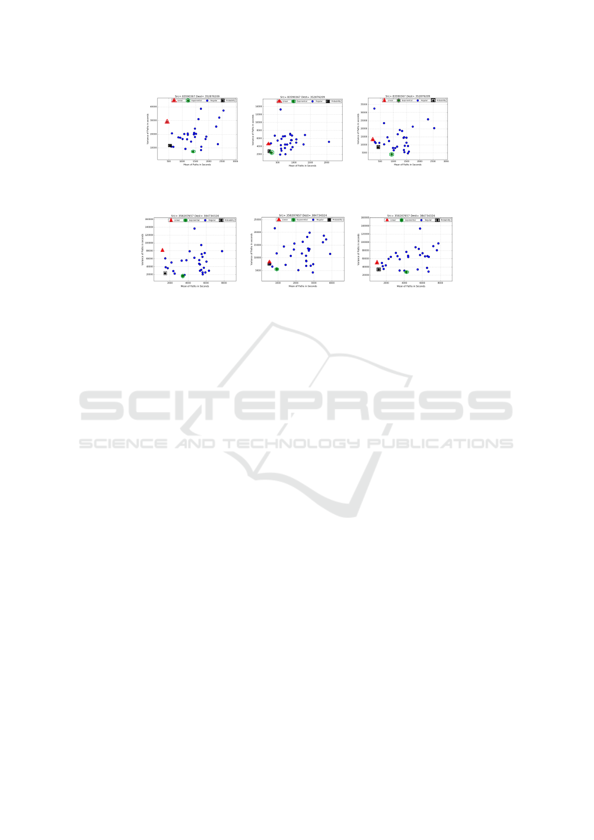
(a) (b) (c)

Figure 5: Selected paths for times of Friday for Source node=83590367 and Destination node=352876209 for each cost

function. Query times from left to right the times are: a) 8:00, b) 15:00, and c) 18:10 PM. Deadline is set as 1200 seconds.

(a) (b) (c)

Figure 6: Selected paths for different times of Tuesday for Source=358207657 and Destination=384734324 for each cost

function. Query times from left to right are: a) 7:30, b) 11:40, and d) 17:45. Deadline is set as 1400 seconds.

4.1.2 Shortest En-route Time

In this experiment, the agent wants to have the short-

est en-route time within a desired arrival interval. We

determine the best time to start the trip and which

path yields the shortest travel time. Figure 7 and Fig-

ure 8, show the results of this experiment for three dif-

ferent time slots of Monday and Wednesday for two

different sets of nodes with all three mentioned cost

functions. Each circle represents one of the paths be-

tween the source and destination. In each ﬁgure, pink

rectangle represents the path with smallest travel time

with the step cost function, green trapezoid is the best

path if the cost function is exponential, and red tri-

angle is the best path based on linear cost function

model.

Similar to the ﬁndings in the previous experiment,

Figure 7 and Figure 8 shows that in rush hours se-

lected paths for different models differ from each

other signiﬁcantly, while in non-peak hours they are

almost the same. It emphasizes the effect of conges-

tion in busy hours and how it changes the weights on

edges of the graphs and impacts the path selection.

As in the previous experiment, the linear model picks

the path with smallest mean, while that path might

have a high variance like Figure 7.(b). Exponential

path does not consider deadline and it may pick a path

which does not make the trip within the desired ar-

rival. Step cost function which provides the shortest

en-route time path considers mean, variance, and de-

sired arrival time. Desired probability for this experi-

ment is considered as 85 percent. This means that we

are interested to ﬁnd the paths that have the smallest

travel time and within the chance of 85 percent can

make the trip before deadline (85 percent is a number

we picked to keep the experiments consistent here, it

can be any probability).

Another ﬁnding indicates that picking the shortest

en-route path sometimes is a risky decision as it has a

high variance of reaching destination before deadline.

For example, in Figure 7 and Figure 8 the smallest

travel time path has the higher variance in comparison

to the path with exponential cost function.

4.2 How Do Selected Paths Compare

with Shortest-length Path?

In the realm of path planning, shortest-length path

is always a practical option. Hence we used it as a

baseline to see how our paths are different from the

shortest-length path. In this experiment, we com-

pare means and variances of shortest-length path with

highest probability path and shortest en-route time

path for 100 random pairs of source and destinations

with the distance of 10 to 12 miles in different areas

of Salt Lake City during morning rush hours. The re-

sults for each of the goals are averaged over all 100

pairs in weekdays (Monday through Friday). Desired

travel time for the pairs is considered as 2200 seconds

(based on the average time takes to get from a source

to destination with the distance for 10 to 12 miles in

rush hour) and desired probability for this experiment

is considered as 85 percent. Figure 9 is the demonstra-

tion of means and variances for each day of the week.

As it can be seen from the graphs, shortest-length path

is not performing well as it just tries to pick the mini-

ICAART 2021 - 13th International Conference on Agents and Artiﬁcial Intelligence

954

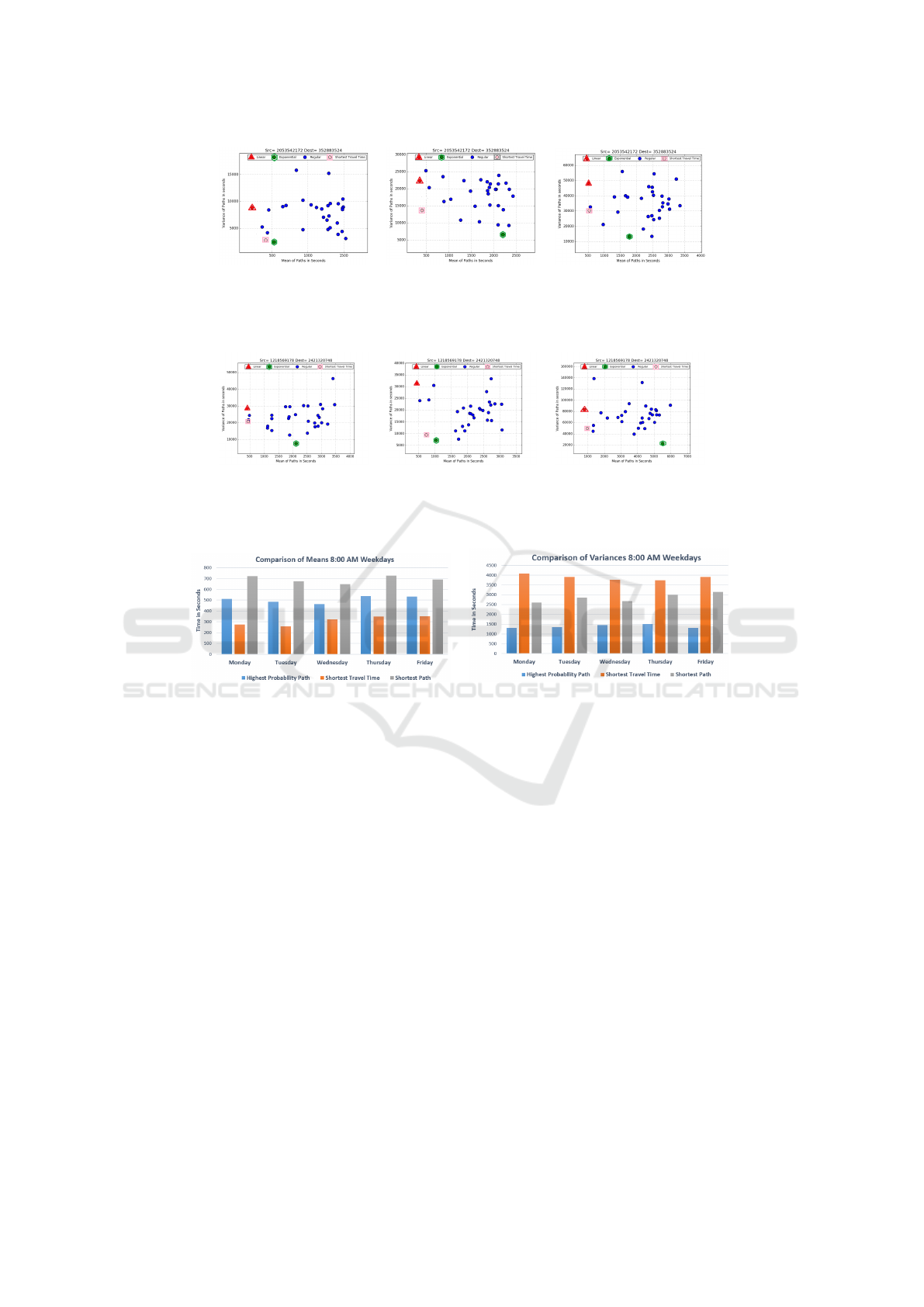
(a) (b) (c)

Figure 7: Selected paths for different times of Monday for Source=2053542172 and Destination=352883524. Times from left

to right are: a) 6:40, b) 8:10, and d) 18:00. Desired arrival time is within the 1600 seconds after query time. Best time for

start the trip to have the smallest travel time is as follow: a) 6:40, b) 8:23, and c) 18:21.

(a) (b) (c)

Figure 8: Selected paths for different times of Wednesday for Source=1218569178 and Destination=2421320748. Times from

left to right are: a) 7:40, b) 11:10, and d) 17:30. Desired arrival time is within the 2000 seconds after query time. Best time

for start the trip to have the smallest travel time is as follow: a) 8:01, b) 11:10, and c) 18:09.

(a) (b)

Figure 9: Comparison of average mean and variance of highest probability path, shortest en-route path and shortest-length

path in 8:00 AM of Weekdays for 100 different source and destinations.

mized length path even if it is congested. Shortest en-

route time paths have smaller means in comparison

to highest probability paths while they have higher

variance which makes highest probability paths more

secure options but longer travel time. Even though

shortest-length paths have reasonable variance, their

high mean value makes them not a good option to

pick.

5 CONCLUSION AND FUTURE

WORK

This research represents path planning in the real

world domain in which edge weights are not ﬁxed

but are stochastically affected by the time of the

day/week. Inspired by time-dependent trafﬁc situ-

ation, we parameterize these distributions by time,

which allows us to speak of time-dependent path costs

and study the problems of reaching a goal by a dead-

line, and delaying departure to minimise traversal-to-

goal time. The best path is the path with lowest cost

and the cost is based on travel time which highly de-

pends on the level of congestion in different time of

the day/week. Since the graph is interconnected, op-

timizing for lowest cost on all possible paths is not

feasible, therefore, we propose a pruning technique to

shrink the search region. Agents can pursue two main

goals: 1) picking the least risky path and 2) picking

the smallest travel time along with awareness of when

to start the trip.

Results show that during rush hour, utilizing an

intelligent path planning approach is crucial. In ad-

dition, we demonstrate that a suitable path planning

approach must consider path’s mean, path’s variance,

agents’ goals and the deadline to provide optimal op-

tions. We also compared the mean and variance of

highest probability paths and shortest en-route paths

with shortest-length paths at the same query time.

This experiment proves that during rush hour shortest-

Congestion-Aware Stochastic Path Planning and Its Applications in Real World Navigation

955

length path is not a good option. Another ﬁnding in-

dicates that, highest probability path has less variance

as it takes the most secure path, while the smallest

travel time has the lowest mean and might have a high

variance.

Possible future work is to consider salable ap-

proaches that enables this framework to handle large

number of path planning queries at the same time.

Also, we can expand the model to offer paths that are

optimal for alleviating the overall congestion of the

city rather than just the best path for each agent (opti-

mal decisions versus selﬁsh decisions).

REFERENCES

Ahmadi, K. and Allan, V. H. (2017). Stochastic Path Find-

ing under Congestion. In 2017 International Confer-

ence on Computational Science and Computational

Intelligence (CSCI), pages 135–140.

Bachman, G., Narici, L., and Beckenstein, E. (2000).

Fourier and Wavelet Analysis. Universitext. Springer

New York, New York, NY.

Campbell, A. M., Gendreau, M., and Thomas, B. W.

(2011). The orienteering problem with stochastic

travel and service times. Annals of Operations Re-

search, 186(1):61–81.

Cao, Z. (2017). Maximizing the probability of arriving on

time : a stochastic shortest path problem.

Chiabaut, N., Buisson, C., and Leclercq, L. (2009). Fun-

damental Diagram Estimation Through Passing Rate

Measurements in Congestion. IEEE Transactions on

Intelligent Transportation Systems, 10(2):355–359.

Dijkstra, E. W. and W., E. (1959). A note on two problems

in connexion with graphs. Numerische Mathematik,

1(1):269–271.

Edler, D., Guedes, T., Zizka, A., Rosvall, M., and Antonelli,

A. (2017). Infomap Bioregions: Interactive Mapping

of Biogeographical Regions from Species Distribu-

tions. Systematic Biology, 66(2):197–204.

Fan, Y. Y., Kalaba, R. E., and Moore, J. E. (2005). Arriving

on Time. Journal of Optimization Theory and Appli-

cations, 127(3):497–513.

Garza, S. E. and Schaeffer, S. E. (2019). Community detec-

tion with the Label Propagation Algorithm: A survey.

Physica A: Statistical Mechanics and its Applications,

534:122058.

Geisberger, R., Kobitzsch, M., and Sanders, P. (2010).

Route planning with ﬂexible objective functions.

Haklay, M. and Weber, P. (2008). OpenStreetMap: User-

Generated Street Maps. IEEE Pervasive Computing,

7(4):12–18.

Hart, P. E., Nilsson, N. J., and Raphael, B. (1968). A for-

mal basis for the heuristic determination of minimum

cost paths. IEEE Transactions on Systems Science and

Cybernetics, 4(2):100–107.

Lau, H. C., Yeoh, W., Varakantham, P., and Nguyen, D. T.

(2012). Dynamic Stochastic Orienteering Problems

for Risk-Aware Applications. Uncertainty in Artiﬁcial

Intelligence: Proceedings of the Twenty-Eighth Con-

ference: August 15-17 2012, Catalina Island, United

States.

Long, D., ICAPS 2006 (16 2006.06.06-10 Windermere, U.,

and International Conference on Automated Planning

and Scheduling (16 2006.06.06-10 Windermere, U.

(2006). Optimal route planning under uncertainty.

AAAI Press.

Miller-Hooks, E. D. and Mahmassani, H. S. (2000). Least

Expected Time Paths in Stochastic, Time-Varying

Transportation Networks. Transportation Science,

34(2):198–215.

Niknami, M. and Samaranayake, S. (2016). Tractable

Pathﬁnding for the Stochastic On-Time Arrival Prob-

lem. pages 231–245. Springer, Cham.

Nikolova, E. and Karger, D. R. (2008). Route Planning un-

der Uncertainty: The Canadian Traveller Problem.

Pi, X. and Qian, Z. S. (2017). A stochastic optimal control

approach for real-time trafﬁc routing considering de-

mand uncertainties and travelers’ choice heterogene-

ity. Transportation Research Part B: Methodological,

104(Supplement C):710 – 732.

Ruaridh Clark, M. M. (2018). Eigenvector-based commu-

nity detection for identifying information hubs in neu-

ronal networks | bioRxiv.

Rus, S. L. B. K. G. R. M. (2020). Method and apparatus for

trafﬁc-aware stochastic routing and navigation.

Sigal, C. E., Pritsker, A. A. B., and Solberg, J. J. (1980).

The Stochastic Shortest Route Problem. Operations

Research, 28:1122–1129.

Wilkie, D., Van Den Berg, J., Lin, M., and Manocha, D.

(2011). Self-Aware Trafﬁc Route Planning.

Yang, Z., Algesheimer, R., and Tessone, C. (2016). A

Comparative Analysis of Community Detection Algo-

rithms on Artiﬁcial Networks. Scientiﬁc Reports, 6.

Yaoxin Wu, Wei Chen, Xuexi Zhang, and Guangjun Liao

(2016). Improving the performance of arrival on time

in stochastic shortest path problem. In 2016 IEEE

19th International Conference on Intelligent Trans-

portation Systems (ITSC), pages 2346–2353. IEEE.

ICAART 2021 - 13th International Conference on Agents and Artiﬁcial Intelligence

956