
Analysis of the Hiring Cost Impact with a Bi-objective Model for the
Multi-depot Open Location Routing Problem
Joel-Novi Rodríguez-Escoto
a
, Samuel Nucamendi-Guillén
b
and Elias Olivares-Benitez
c
Facultad de Ingeniería, Universidad Panamericana, Álvaro del Portillo 49, Zapopan, México
Keywords: Location-routing Problem, Multi-objective Optimization, Exact Methods, AUGMECON2, Goal
Programming, Heterogeneous Fleets.
Abstract: This paper investigates the effect of the hiring cost over transportation cost and the capacity utilization for the
vehicles used. This analysis is conducted on a multi-depot open location-routing problem. The problem
consists of determining the optimal number of depots to open, as well as the design of the open routes in order
to satisfy the demand for all of the customers while seeking the best trade-off between the total traveling and
opening cost. To solve the problem, we propose a bi-objective mixed-integer linear model, which is solved
using two different approaches: the augmented epsilon constraint 2 (AUGMECON2) method and the
weighting revised multi-choice goal programming (WRMCGP) method. Both approaches are implemented,
solving benchmark instances and comparing the quality of the Pareto fronts in terms of multi-objective metrics.
Accordingly, the results indicate that AUGMECON2 performs better than WRMCGP concerning the quality
of the Pareto Front and the elapsed CPU time, for instances with a homogeneous fleet. However, the
WRMCGP reported the best solution time in the heterogeneous instances. In summary, considering
heterogeneous fleets, the results demonstrate that the hiring cost can be reduced up to 85%, with 73% more
vehicle utilization on average.
1 INTRODUCTION
The vehicle routing problem (VRP) is one of the most
studied problems in Operations Research due to the
diverse applications where it can be implemented. Its
practical relevance and theoretical complexity make
this topic so attractive, as this provides solutions to
several kinds of logistics and transportation problems
(Elshaer & Awad, 2020; Irnich et al., 2014; Kardar et
al., 2011). A particular variant of the VRP, known as
the multi-depot location-routing problem
(MDOLRP), determines the number of depots to
open, the location of those depots, and the routes'
design simultaneously. The problem studied in this
work is inspired by the situation faced by a Mexican
company, which imports material from suppliers in
the USA. The firm agrees with a third-party company
an exclusive contract transport the raw material. This
translates into high costs. The reason for the high cost
comes from the supplier agreement since it requires
a
https://orcid.org/0000-0002-8687-6809
b
https://orcid.org/0000-0003-4169-3395
c
https://orcid.org/0000-0001-7943-3869
to contract a homogeneous fleet. The company is
interested in analyzing the hiring of different
transportation suppliers and considering a
heterogeneous fleet. Given the specific context, the
MDOLRP can be used to solve the problem. The
purpose is to determine the impact of hiring costs over
the total cost. In the single-objective version of this
problem (Nucamendi-Guillén et al., 2020), the
authors focused on minimizing the total incurred cost
expressed as the sum of the traveling and vehicle’s
hiring cost. However, the study did not evaluate the
effect of the hiring cost over the traveling cost. The
purpose of this work is to conduct a bi-objective
analysis to show if reducing the number of vehicles
used forces to create routes that increase the cost
significantly.
The present study follows two objectives: (i) to
solve the bi-objective problem model with exact
methods, and (ii) to solve and compare the
performance of each solution method based on the
Rodríguez-Escoto, J., Nucamendi-Guillén, S. and Olivares-Benitez, E.
Analysis of the Hiring Cost Impact with a Bi-objective Model for the Multi-depot Open Location Routing Problem.
DOI: 10.5220/0010266604250432
In Proceedings of the 10th International Conference on Operations Research and Enterprise Systems (ICORES 2021), pages 425-432
ISBN: 978-989-758-485-5
Copyright
c
2021 by SCITEPRESS – Science and Technology Publications, Lda. All rights reserved
425

quality of the Pareto fronts, using multi-objective
metrics. In addition, the analysis of the costs between
homogeneous and heterogeneous fleets is conducted.
The remainder of the paper is organized as
follows. Section 2 presents the literature review of the
MDOLRP. Section 3 describes the multi-objective
optimization model, the solution methods, and the
characteristics of the set of instances. Section 4
reports the results obtained, including the comparison
with the multi-objective metrics and the hiring cost
analysis. Finally, the concluding remarks of this work
are presented in section 5.
2 LITERATURE REVIEW
The location-routing problem (LRP) is a
generalization of the VRP in which the optimal
number of open depots and optimal design of the
routes are simultaneously determined (Wu et al.,
2002). As a generalization of the VRP, the LRP is
considered as an NP-hard problem. Because of this, it
is difficult to obtain optimal solutions to large
instances in reasonable computational time, justifying
the use of metaheuristics (Adhi et al., 2019; Rabbani
et al., 2017). Nevertheless, small instances can be
solved with exact methods, with standard
computational capacity and enough time to solve
(Braekers et al., 2016; Ramos et al., 2014).
In the LRP, the selection of the depot represents a
strategical decision, while the design of the routes is
an operational decision. However, additional features
can affect the decision of location and routing, for
instance, to have a limit in the number of depots to
open or when facilities have limited capacity
(Schneider & Drexl, 2017). Finally, the characteristic
of considering open routes denote that the vehicle is
not required to return to the depot after visiting the
last customer, which is common when a third party
executes the distribution since they assume the cost
of the "empty" return (Braekers et al., 2016).
The single objective approach of the location-
routing problem usually requires minimizing a
combination, sometimes weighted, of fixed and
variable costs. Differently, the multi-objective
approach optimizes conflicting objectives, for
instance, minimizing the travel cost and maximizing
the level of service (Drexl & Schneider, 2015;
Tavakkoli-Moghaddam et al., 2010). When the
conflicting objectives belong to different dimensions,
a normalization process is performed before
implementing the model.
One of the methods commonly used is weighted
goal programming (WGP), which has been
previously applied in multi-objective location-routing
problems (Zhao & Verter, 2015; Rabbani et al., 2017;
Asefi et al., 2019; Yousefi et al., 2017).
In the specific case of bi-objective problems, the
Epsilon-constraint method arises as an approach to be
applied in multi-objective routing problems
(Kabadurmus et al., 2019; Toro et al., 2017; Arango
González et al., 2017). An improved version of the ε-
constraint, the augmented epsilon-constraint method
(AUGMECON) has gained researchers' attention to
solve multi-objective routing problems (Wang et al.,
2018; Amini et al., 2019).
The literature review illustrates the tendency to
solve realistic routing problems via exact multi-
objective methods, from the weighting method,
weighting goal programming, to epsilon-constraint
based method. These techniques optimize objectives
that belong to different nature and in quantity, even if
they are conflicting. Even when, in general, the WGP
and its variations are frequently used to solve multi-
objective routing problems, they present
complications when solving large-scale instances,
justifying the use of methods as the ones proposed in
the present work, which are enough to solve and
analyze the bi-objective location-routing problem.
3 MATHEMATICAL MODEL AND
SOLUTION METHODS
This work provides a detailed analysis of the bi-
objective version of the MDOLRP (Nucamendi-
Guillén et al., 2020), following two different
strategies. The details and characteristics of the
problem, the assumptions, and the model formulation
are presented next. The MDOLRP model is
functional to analyze the impact of hiring cost in
minimizing the total cost. For practical purposes, the
following assumptions are made:
The routes generated should be finished in the
manufacturing company;
The return cost of the supplier transport to the
depot is considered on the hiring cost. It means
the open routes;
The demand is deterministic and quantified in
pallets;
The traveled distance is translated into
monetary terms.
3.1 Problem Definition
The following notation is used:
𝑛 ∶ 𝑁𝑢𝑚𝑏𝑒𝑟 𝑜𝑓 𝑠𝑢𝑝𝑝𝑙𝑖𝑒𝑟𝑠
𝑚 ∶ 𝑁𝑢𝑚𝑏𝑒𝑟 𝑜𝑓 𝑐𝑎𝑟𝑟𝑖𝑒𝑟𝑠
ICORES 2021 - 10th International Conference on Operations Research and Enterprise Systems
426

𝑄
∶ 𝑀𝑎𝑥𝑖𝑚𝑢𝑚 𝑐𝑎𝑝𝑎𝑐𝑖𝑡𝑦 𝑝𝑒𝑟 𝑎𝑛𝑦 𝑣𝑒ℎ𝑖𝑐𝑙𝑒
𝑤
∶ 𝐻𝑖𝑟𝑖𝑛𝑔 𝑐𝑜𝑠𝑡 𝑝𝑒𝑟 𝑣𝑒ℎ𝑖𝑐𝑙𝑒 𝑙 𝑝𝑒𝑟 𝑐𝑎𝑟𝑟𝑖𝑒𝑟 𝑖
𝐷
: 𝑇𝑟𝑎𝑛𝑠𝑝𝑜𝑟𝑡 𝑐𝑜𝑠𝑡 𝑏𝑒𝑡𝑤𝑒𝑒𝑛 𝑑𝑒𝑝𝑜𝑡 𝑖 𝑎𝑛𝑑 𝑠𝑢𝑝𝑝𝑙𝑖𝑒𝑟 𝑗
𝐶
: 𝑇𝑟𝑎𝑛𝑠𝑝𝑜𝑟𝑡 𝑐𝑜𝑠𝑡 𝑏𝑒𝑡𝑤𝑒𝑒𝑛 𝑠𝑢𝑝𝑝𝑙𝑖𝑒𝑟𝑠 𝑖 𝑎𝑛𝑑 𝑗
Let 𝑃1,..,𝑛1, be the set that denotes the
nodes to visit. Let 𝑃𝑝1,..,𝑛, the node-set for the
suppliers (where n represents the number of suppliers
to serve) to collect whereas the node 𝑛1 denotes
the final node (i.e., the manufacturing plant). Let 𝐹
1,…,𝑚 be the set of potential carriers (where m
represents the number of carriers to contract), where
𝑅
1,…,𝑘
denotes the set of vehicles per each
carrier, where 𝑘
represents the number of vehicles
per each carrier. The capacity and the hiring cost of
each vehicle 𝑙 belonging to carrier 𝑖 are denoted as 𝑄
and 𝑤
, respectively. The demand per supplier 𝑗 is
in 𝑑
. The transport cost is due to the next matrix:
depot 𝑖 to supplier 𝑗 is in 𝐷
, and supplier 𝑖 to
supplier 𝑗 is in 𝐶
.
Regarding the variable set, let 𝑜
be a binary
variable equal to 1, if the arc 𝑖,𝑗 is active to travel
from the depot 𝑖 and the first node 𝑗 using the
vehicle 𝑙, and equal to 0 otherwise. Let 𝑥
be a binary
variable equal to 1, if the arc 𝑖,𝑗 is traveled between
nodes 𝑖 and 𝑗, and equal to 0 otherwise. Let 𝑧
be
equal to 1, if vehicle 𝑙 is contracted from the carrier 𝑖,
and equal to 0 otherwise. Furthermore, let the
auxiliary variable 𝑣
be a continuous variable that
denotes the sum of the demands of the remaining
nodes of the route after departing from carrier 𝑖 using
vehicle 𝑙 when 𝑜
1. In addition, let the
auxiliary variable 𝑟
be a continuous variable that
denotes the sum of the demands of the remaining
nodes of the route after visiting supplier 𝑖 when 𝑥
1.
Since this work aims to analyze the impact of the
hiring cost (𝐹2) above the traveling cost (𝐹1), the
objective is conflicted naturally, as proportionally
contrary to the problem. The bi-objective model
approach is addressed. The mathematical formulation
is:
𝐹1𝑚𝑖𝑛𝐷
𝑜
𝐶
𝑥
,
(1)
𝐹2𝑚𝑖𝑛𝑤
𝑧
(2)
Subject to:
𝑜
1,∀𝑖 ∈𝐹;𝑙∈𝑅
,
(3)
𝑜
𝑥
1,∀ 𝑗 ∈𝑃𝑝,
(4)
𝑥
1,∀𝑗 ∈𝑃𝑝,
(5)
𝑧
𝑜
,
∀𝑖 ∈𝐹;𝑙∈𝑅
,
(6)
𝑣
𝑑
𝑜
,∀𝑖 ∈𝐹;𝑗∈𝑃𝑝; 𝑙∈𝑅
,
(7)
𝑣
𝑄
𝑜
,∀𝑖 ∈𝐹;𝑗∈𝑃𝑝; 𝑙∈𝑅
,
(8)
𝑟
𝑑
𝑥
,∀𝑖∈𝑃𝑝;𝑗∈𝑃𝑝; 𝑖𝑗,
(9)
𝑟
𝑄
𝑑
𝑥
,∀𝑖∈𝑃𝑝;𝑗∈𝑃𝑝; 𝑖𝑗,
(10)
𝑣
𝑟
𝑟
𝑑
,∀ ℎ ∈𝑃𝑝,
(11)
𝑜
∈
0,1
,∀𝑖 ∈𝐹;
𝑗
∈𝑃𝑝; 𝑙∈𝑅
,
(12)
𝑥
∈
0,1
,∀𝑖∈𝑃𝑝;
𝑗
∈𝑃,
(13)
𝑧
∈
0,1
,∀𝑖 ∈𝐹;𝑙∈𝑅
,
(14)
𝑣
0,∀𝑖 ∈𝐹;
𝑗
∈𝑃𝑝; 𝑙∈𝑅
,
(15)
𝑟
0,∀𝑖∈𝑃𝑝;
𝑗
∈𝑃.
(16)
The objective functions (1) and (2) minimizes the
sum of the transportation and contracting costs,
respectively. Constraints (3) ensure that, for each
vehicle, at most, one departing arc must be activated.
In contrast, the group of constraints (4) assure each
supplier node must be visited only once, either from
the depot or from other nodes. Constraints (5) ensure
that all of the routes end at node n+1. The constraints
(6) activates the carriers for the selected vehicles
(departing nodes). On the other hand, constraints (7)
ensure that the demand of each departing node must
be satisfied. Also, the constraints (8) ensure that the
cumulative demand of each route does not exceed the
capacity 𝑄
. Constraints (9) and (10) operate in the
same way as (7) and (8) but involving only the
supplier nodes. Constraints (11) avoid having sub-
tours by controlling demand. Finally, constraints
(12)-(16) denote the nature of the variables.
Since this study aims to analyze the behavior of
the vehicles' hiring and traveling cost over the total
cost, for both the case of the heterogeneous and
Analysis of the Hiring Cost Impact with a Bi-objective Model for the Multi-depot Open Location Routing Problem
427
homogeneous fleet, it is necessary to use the multi-
objective optimization method. This optimization
approach is useful to manage decision-making
problems involving two or more conflicting
objectives. Given the characteristics of the problem,
this procedure is followed.
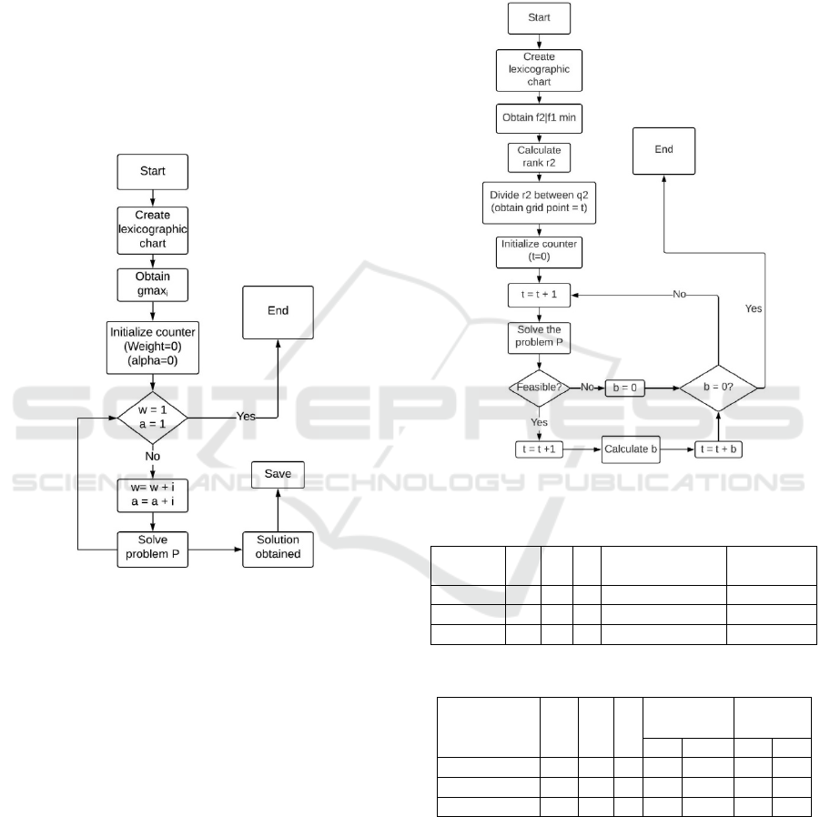
3.2 Solution Methods
The computational experiments were executed using
both approaches, WRMCGP and AUGMECON2.
Figure 1 describes the implementation of WRMCGP.
Figure 2 exhibits the implementation of
AUGMECON2.
Figure 1: WRMCGP diagram.
4 COMPUTATIONAL
EXPERIENCE
4.1 Set of Instances
For computational experimentation, we considered
two different sets of instances. The first set belongs to
the instances used for the multi-depot vehicle routing
problem, proposed in (Cordeau et al., 1997) and
labeled P and Pr. The second set involves the
instances with a heterogeneous fleet (Wang & Wu,
2015). For the heterogeneous instances, different
opening costs per each depot were considered. In the
instances involving a homogeneous fleet, all the
vehicles have the same opening cost.
After implementing the model, only three
instances of each group could be entirely solved (six
in total). Tables 1 and 2 indicate the description of
those instances. In these tables, columns 1-5 indicate
the name of the instance, number of suppliers (n),
number of depots (m), number of vehicles (k), and
vehicles' hiring costs, respectively.
Figure 2: AUGMECON2 diagram.
Table 1: Description of the homogeneous instances.
Instance
name
n m k
Vehicle
ca
p
acit
y
Hiring
cost
P_02 50 4 5 160 31.80
Pr_01 48 4 4 200 63.13
Pr
_
02 96 4 7 195 60.70
Table 2: Description of the heterogeneous instances.
Instance
name
n m k
Vehicles
Capacities
Hiring
costs
min max min max
Wa-W15O1 20 2 15 4 8 20 35
Wa-W15O2 24 3 15 4 5 15 20
Wa-W15O3 25 3 15 4 5 15 20
The formulation was coded using the optimization
language AMPL and solved using Gurobi 9.0.0 using
computational equipment with an Intel Core i7-
6600U @ 2.6GHz processor with 16 GB of RAM,
under Windows 10 as OS. The computational time
limit is set to 7200 seconds per iteration in the Pareto
Front.
ICORES 2021 - 10th International Conference on Operations Research and Enterprise Systems
428
4.2 Multi-objective Metrics
To measure the performance of the method, we use
the following metrics:
NOS/NPS:
The number of optimal solutions in the Pareto
Front evidences the best performance between
algorithms; a higher NPS value is preferred (Rayat et
al., 2017).
Quality metric (QM):
This metric calculates the proportion between the
number of non-dominated Pareto Front solutions of
method A and the total non-dominated solutions from
the combined Pareto front (Rayat et al., 2017), as
shown in equation (17).
𝑄
𝐴
𝑁𝑢𝑚𝑏𝑒𝑟 𝑜𝑓 𝑛𝑜𝑛 𝑑𝑜𝑚𝑖𝑛𝑎𝑡𝑒𝑑 𝑠𝑜𝑙𝑢𝑡𝑖𝑜𝑛𝑠 𝑜𝑓 𝑚𝑒𝑡ℎ𝑜𝑑 𝐴
𝑇𝑜𝑡𝑎𝑙 𝑛𝑢𝑚𝑏𝑒𝑟 𝑜𝑓 𝑛𝑜𝑛
_
𝑑𝑜𝑚𝑖𝑛𝑎𝑡𝑒𝑑 𝑠𝑜𝑙𝑢𝑡𝑖𝑜𝑛𝑠
,
(17)
The quality of solutions is compared against each
other, and the higher value algorithm is desirable.
RPOS:
The metric determines the ratio of Pareto-optimal
solutions in 𝑃
that are not dominated by any other
solutions in 𝑃, which is the union of the sets of the
Pareto-optimal solution, and it is calculated using
equation (18) (Altiparmak et al., 2006):
𝑅𝑃𝑂𝑆
𝑃
|
𝑃
𝑋
∈𝑃
|∃ 𝑌∈𝑃∶ 𝑌≺
𝑋
|
|
𝑃
|
(18)
Where
𝑌≺𝑋 means the solution 𝑋 is dominated
by the solution
𝑌, and these solutions 𝑋 are removed
from the solution set
𝑃
. The higher value, the better.
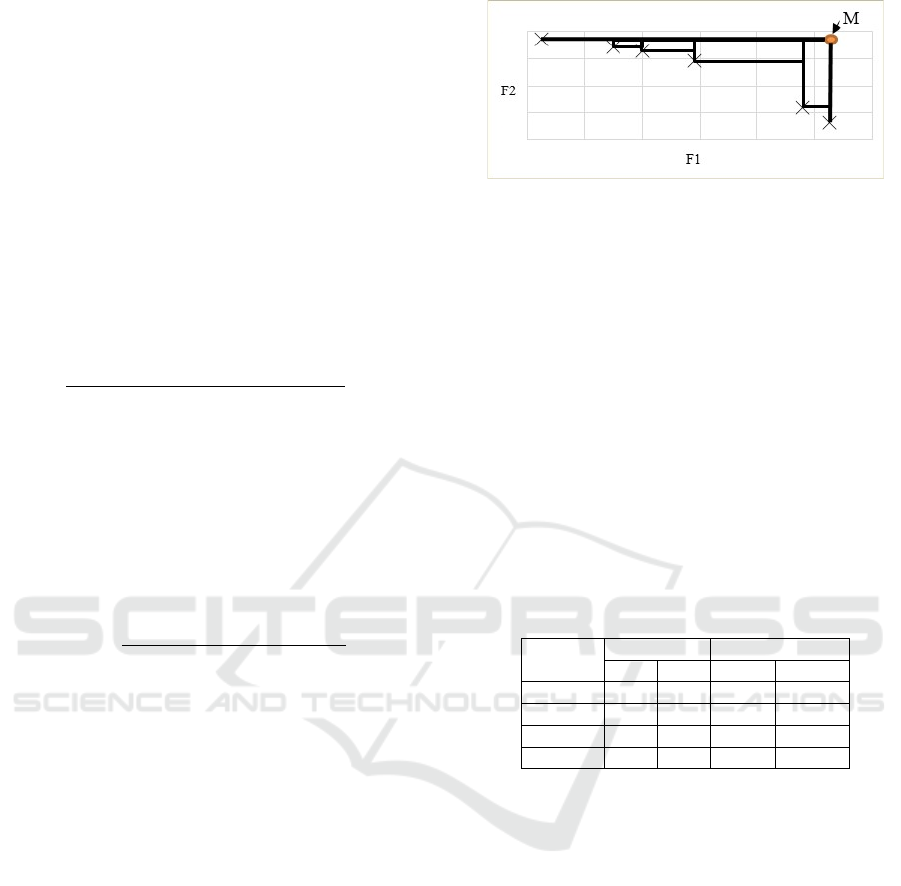
Hyperarea ratio (HR):
The proportion of the generated area (HR) (21) is
calculated by dividing the Pareto front area (HA) for
each point between the total area (TA) (Zitzler &
Thiele, 1999), as shown in eq. (21). The area (HA) of
the Pareto Front can be defined as the product of the
difference between coordinate (𝐹1
, 𝐹2
) for each
solution 𝑆
and the (highest) maximum point (M), as
defined in eq. (19). Lastly, the total area (TA) is the
product of the difference between the coordinates
(𝑀, 𝐹1
), and (𝑀,𝐹2
) (20). Figure 3 shows an
example to calculate Hyperarea of a Pareto front.
𝐻𝐴
𝑓
1
𝑓
1
∗
𝑓
2
𝑓
2
,
(19)
𝑇𝐴
𝑓
2
𝑓
2
∗
𝑓
1
𝑓
1
,
(20)
𝐻𝑅 𝐻𝐴 𝑇𝐴
⁄
,
(21)
Figure 3: Hyperarea of the Pareto front.
4.3 Experimental Results
This section is devoted to reporting the values of the
metrics used to evaluate each method's efficiency
over each specific group of instances. First, the values
of the NPS and elapsed CPU time is shown. Then, the
values of the Q(A), RPOS, and HR are displayed.
Tables 3 and 4 report the value of NPS and the
CPU time (in seconds) for each solution approach
over each type of instance. These two metrics are first
considered since they quickly indicate the method's
performance in terms of quality and speed. The
columns are identified with an (A) for
AUGMECON2 and a (W) for WRMGCP.
Table 3: NPS and computational time of optimality
homogeneous instances.
Instance
name
NPS CPU Time
(
sec
)
AW A W
P_02 5 8 1054 10373
Pr_01 9 6 34 44
Pr_02 5 3 3108 5023
Avera
g
e 6.33 5.67 1398 5146
It is evident that AUGMECON2 performs better
than WRMCGP, reporting denser fronts in general
and in the case of the homogeneous instances,
requiring 74.76 % less time on average than
WRMCGP. On the other hand, there is a difference of
65.69% on average in the heterogeneous instances in
favor of WRMCGP. Since the number of points in the
Front differs per method, a detailed analysis is
conducted to determine the variation between the
minimum and maximum values for the extreme
solutions of each Pareto Front. This analysis is shown
in section 4.4.
The next analysis consists of determining which
method produces better Pareto fronts with respect to
the remaining metrics Q(A), RPOS, and HR. Tables
5 and 6 show the values obtained for the
heterogeneous and homogeneous instances,
respectively. The columns are identified with an (A)
for AUGMECON2 and a (W) for WRMGCP.
Analysis of the Hiring Cost Impact with a Bi-objective Model for the Multi-depot Open Location Routing Problem
429
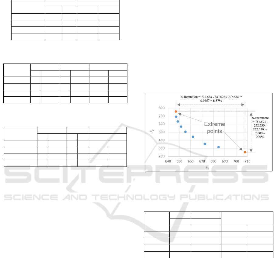
Table 4: NPS and computational time of optimality-solved
heterogeneous instances.
Instance
name
NPS CPU Time (sec)
A W A W
Wa-W15O1 6 5 611 276
Wa-W15O2 4 3 3126 1217
Wa-W15O3 3 3 996 129
Avera
g
e 4.33 3.67 1578 541
Table 5: Results of multi-objective metrics for the
homogeneous instances.
Instances
Q
(
A
)
RPOS HR
A W A W A W
P_02 1 0.625 1 1 0.699 0.657
Pr_01 1 0.667 1 0.833 0.695 0.657
Pr
_
02 1 0.6 1 1 0.616 0.521
Avera
g
e 1 0.631 1 0.944 0.670 0.612
Table 6: Results of multi-objective metrics for the
heterogeneous instances.
Instances
Q
(
A
)
RPOS HR
A W A W A W
Wa-W15O1 1 0.833 1 1 0.781 0.78
Wa-W15O2 1 0.75 1 1 0.318 0.258
Wa-W15O3 1 1 1 1 0.736 0.736
Avera
g
e 1 0.861 1 1 0.612 0.591
From tables 5 and 6, it can be observed that
AUGMECON2 performs better, improving by 36.9%
in quality, 2.56% in RPOS, and 8.66% in HR for
homogeneous instances and improving by 23.9% in
quality, 0.0% in RPOS, and 3.43% in HR in
heterogeneous instances. In general, AUGMECON2
outperforms WRMCGP, even when WRMCGP
presents a competitive computational time
performance in the heterogeneous instances.
In summary, it was demonstrated that the vehicles'
hiring costs play an essential role when the DM seeks
a better trade-off between the number of vehicles to
hire and the total distance traveled, representing a
metric of customer satisfaction. A detailed analysis is
presented next to better understand the impact of
hiring cost over travel distance and capacity
utilization.
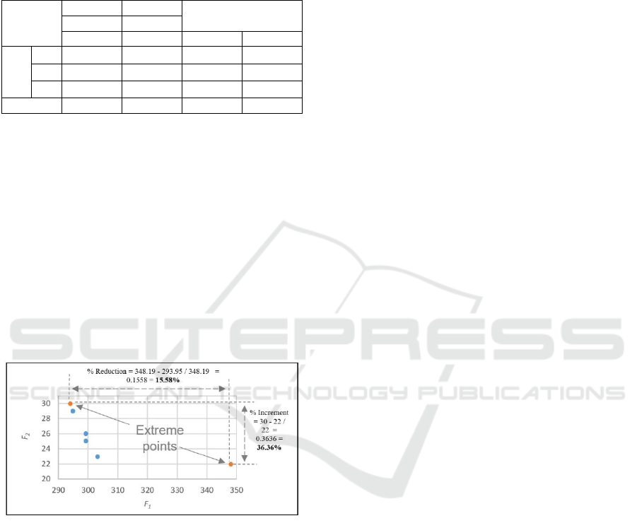
4.4 Detailed Analysis of the Impact of
Vehicles' Hiring Cost
As mentioned before, a detailed analysis is conducted
to evaluate the impact of the hiring cost over the
transportation cost (in both cases) and vehicles'
capacity utilization. This study was performed in two
stages. First, we calculate the proportion of
improvement in the transportation cost (F1) and
hiring cost (F2) as the difference between the Front's
extreme points. Secondly, the capacity utilization per
vehicle was estimated for each extreme point. Figures
4 and 5 illustrate the calculation of these values for
the instances Pr_01 and Wa-W15O1, respectively.
Tables 7 and 8 summarize the percentage of
reduction in transportation and hiring cost over the
homogeneous and heterogeneous fleet instances,
respectively. In these tables, the first column indicates
the name of the instance. In contrast, columns two and
three reports the percentage of reduction (RED) in
transportation and increment (INC) in hiring cost,
respectively. Finally, columns five and six report the
minimum and maximum percentages of capacity
utilization, respectively.
Figure 4: Percentage calculation of cost savings, for
instance Pr_01.
Table 7: Percentage of cost reduction and capacity
utilization for homogeneous instances.
Instance
name
RED INC
% Avg. of Capacity
utilization
T. cost H. cost
F
1
F
2
Min Max
P_02 5.76% 140.00% 37.36% 97.50%
Pr_01 8.57% 200.00% 27.38% 85.13%
Pr_02 2.78% 57.14% 56.88% 93.11%
Avera
g
e 5.70% 132.38% 40.54% 91.91%
The average percentage of increment cost for
homogeneous instances is 132.38% for hiring cost on
average, producing savings of around 5.70% on
average for transportation costs. On the other hand, if
we choose the minimum Hiring cost, this produces an
average increment of 6.12 % in transportation costs.
When analysing the capacity utilization, it raises
from 40.54% to 91.91%, which indicates that looking
for the best solution in distance tends to sub-utilize
the vehicles' capacity. Moreover, when the decision-
maker seeks for seizing the vehicle's capacity
utilization, the total traveled distance is worsened by
less than 10%, but producing increasing in hiring
costs up to two times more, which is significant since,
ICORES 2021 - 10th International Conference on Operations Research and Enterprise Systems
430
for these instances, the contracting costs represent up
to 60% of the total value (transportation + hiring
costs).
Table 8: Percentage of cost reduction and capacity
utilization in heterogeneous instances.
Instance
name
RED INC
% Avg. of Capacity
utilization
T. cost H. cost
F
1
F
2
Min Max
Wa-W15
O1
15.58%
36.36%
72.74% 96.00%
O2
11.02%
10.00%
92.86% 100%
O3
7.42%
12.50%
87.62% 98.57%
Avera
g
e 11.34% 19.62% 84.41% 98.19%
In the instances with the heterogeneous fleet, it was
observed that savings in transportation costs raised to
11.34% while, for the hiring costs, the increment is
around 15.62%, on average. On the other hand, if we
choose the Hiring cost minimum, this provokes an
average increment of 12.95% in the transport cost. As
a conclusion, it can be observed that it is more rentable
to have different carriers (heterogeneous) to sacrifice
long travel and more vehicle utilized. When having
vehicles with different capacities, the model seeks a
better combination. It can also be confirmed when
observing the minimum and maximum values for
capacity utilization because vehicles have a
utilization of over 70% in the worst case.
Figure 5: Percentage calculation of cost savings for instance
Wa-W15O1.
In summary, considering that contracting costs
represent up to 40% of the total cost, we can initially
conclude that seizing vehicles utilization should be
preferred over total traveling distance for routing
problems involving hiring costs.
5 CONCLUSIONS AND FUTURE
RESEARCH
This work analyzes the impact of the hiring cost over
the transportation cost through a bi-objective model
for the MDOLRP, considering vehicles with a
homogeneous and heterogeneous fleet. The problem
was modeled using a bi-objective model and solved
using a commercial solver, testing literature instances
and obtaining optimality for instances up to 25
suppliers, 2 to 3 depots, and 15 vehicles for the
heterogeneous fleet and, in the case of the
homogeneous fleet, instances up to 96 suppliers, 4
depots, and 7 vehicles.
In terms of the methods used, AUGMECON2
outperformed WRMCGP. However, WRMCGP
performed faster in heterogeneous instances. In
addition, we demonstrate that in the heterogeneous
instances, the saving in hiring cost is significant by
maximizing the vehicles' capacity utilization without
significantly affecting transportation costs. In the case
of the homogeneous instances, the savings are less
substantial.
Future work involves the application of
metaheuristic algorithms to deal with large-scale
instances. In addition, the application of different
objectives as max time delivery, customer service
level, priority index, time windows, split delivery,
autonomous vehicles, and drone application can also
be interesting to the academic knowledge.
ACKNOWLEDGEMENTS
This research was supported by Universidad
Panamericana [grant number UP-CI-2020-GDL-07-
ING].
REFERENCES
Adhi, A., Santosa, B., & Siswanto, N. (2019). A new
metaheuristics for solving vehicle routing problem:
Partial Comparison Optimization. IOP Conference
Series: Materials Science and Engineering, 598,
012023. https://doi.org/10.1088/1757-899X/598/1/
012023
Altiparmak, F., Gen, M., Lin, L., & Paksoy, T. (2006). A
genetic algorithm approach for multi-objective
optimization of supply chain networks. Computers &
Industrial Engineering, 51(1), 196-215.
https://doi.org/10.1016/j.cie.2006.07.011
Amini, A., Tavakkoli-Moghaddam, R., & Ebrahimnejad, S.
(2019). A bi-objective transportation-location arc
routing problem. Transportation Letters, 1-15.
https://doi.org/10.1080/19427867.2019.1679405
Arango González, D. S., Olivares-Benitez, E., & Miranda,
P. A. (2017). Insular Bi-objective Routing with
Environmental Considerations for a Solid Waste
Collection System in Southern Chile. Advances in
Analysis of the Hiring Cost Impact with a Bi-objective Model for the Multi-depot Open Location Routing Problem
431

Operations Research, 2017, pp. 1-11.
https://doi.org/10.1155/2017/4093689.
Asefi, H., Shahparvari, S., Chhetri, P., & Lim, S. (2019).
Variable fleet size and mix VRP with fleet
heterogeneity in Integrated Solid Waste Management.
Journal of Cleaner Production, 230, 1376-1395.
https://doi.org/10.1016/j.jclepro.2019.04.250
Braekers, K., Ramaekers, K., & Van Nieuwenhuyse, I.
(2016). The vehicle routing problem: State of the art
classification and review. Computers & Industrial
Engineering, 99, 300-313. https://doi.org/10.1016/
j.cie.2015.12.007
Cordeau, J.-F., Gendreau, M., & Laporte, G. (1997). A tabu
search heuristic for periodic and multi-depot vehicle
routing problems. Networks: An International Journal,
30, 105–119. https://doi.org/10.1002/(SICI)1097-0037
(199709)30:2%3C105::AID-NET5%3E3.0.CO;2-G
Drexl, M., & Schneider, M. (2015). A survey of variants
and extensions of the location-routing problem.
European Journal of Operational Research, 241(2),
283-308. https://doi.org/10.1016/j.ejor.2014.08.030
Elshaer, R., & Awad, H. (2020). A taxonomic review of
metaheuristic algorithms for solving the vehicle routing
problem and its variants. Computers & Industrial
Engineering, 140, 106242. https://doi.org/10.1016/
j.cie.2019.106242
Irnich, S., Toth, P., & Vigo, D. (2014). Chapter 1: The
Family of Vehicle Routing Problems. In P. Toth & D.
Vigo (Eds.), Vehicle Routing (pp. 1-33). Society for
Industrial and Applied Mathematics. https://doi.org/
10.1137/1.9781611973594.ch1
Kabadurmuş, Ö., Erdoğan, M. S., Özkan, Y., & Köseoğlu,
M. (2019). A Multi-Objective Solution of Green
Vehicle Routing Problem. Logistics & Sustainable
Transport, 10 (1), pp. 31-44. https://doi.org/
10.2478/jlst-2019-0003.
Kardar, L., Farahani, R., & Rezapour, S. (2011). Logistics
Operations and Management: Concepts and Models.
Elsevier. http://ebookcentral.proquest.com/lib/upgdl-
ebooks/detail.action?docID=692427
Nucamendi-Guillén, S., Padilla, A. G., Olivares-Benitez,
E., & Moreno-Vega, J. M. (2020). The multi-depot
open location routing problem with a heterogeneous
fixed fleet. Expert Systems with Applications, 113846.
https://doi.org/10.1016/j.eswa.2020.113846
Rabbani, M., Farrokhi-Asl, H., & Asgarian, B. (2017).
Solving a bi-objective location routing problem by a
NSGA-II combined with clustering approach:
Application in waste collection problem. Journal of
Industrial Engineering International, 13(1), 13-27.
https://doi.org/10.1007/s40092-016-0172-8
Ramos, M. A., Boix, M., Montastruc, L., & Domenech, S.
(2014). Multiobjective Optimization Using Goal
Programming for Industrial Water Network Design.
Industrial & Engineering Chemistry Research, 53(45),
17722-17735. https://doi.org/10.1021/ie5025408
Rayat, F., Musavi, M., & Bozorgi-Amiri, A. (2017). Bi-
objective reliable location-inventory-routing problem
with partial backordering under disruption risks: A
modified AMOSA approach. Applied Soft Computing,
59, 622-643. https://doi.org/10.1016/j.asoc.2017.
06.036
Schneider, M., & Drexl, M. (2017). A survey of the
standard location-routing problem. Annals of
Operations Research, 259(1-2), 389-414.
https://doi.org/10.1007/s10479-017-2509-0
Tavakkoli-Moghaddam, R., Makui, A., & Mazloomi, Z.
(2010). A new integrated mathematical model for a bi-
objective multi-depot location-routing problem solved
by a multi-objective scatter search algorithm. Journal
of Manufacturing Systems, 29(2-3), 111-119.
https://doi.org/10.1016/j.jmsy.2010.11.005
Toro, E. M., Franco, J. F., Echeverri, M. G., & Guimarães,
F. G. (2017). A multi-objective model for the green
capacitated location-routing problem considering
environmental impact. Computers & Industrial
Engineering, 110, pp. 114-125, https://doi.org/
10.1016/j.cie.2017.05.013.
Wang, S., Wang, X., Liu, X., & Yu, J. (2018). A Bi-
Objective Vehicle-Routing Problem with Soft Time
Windows and Multiple Depots to Minimize the Total
Energy Consumption and Customer Dissatisfaction.
Sustainability, 10(11), 4257. https://doi.org/10.3390/
su10114257
Wang, T. J., & Wu, K. J. (2015). Optimization algorithm
for multi-vehicle and multi-depot emergency vehicle
dispatch problem. Advances in Transportation Studies,
2, pp. 23-30. https://doi.org/10.4399/97888548896
3703
Wu, T.-H., Low, C., & Bai, J.-W. (2002). Heuristic
solutions to multi-depot location-routing problems.
Computers & Operations Research, 29(10), 1393-
1415. https://doi.org/10.1016/S0305-0548(01)00038-7
Yousefi, H., Tavakkoli-Moghaddam, R., Taheri Bavil
Oliaei, M., Mohammadi, M., & Mozaffari, A. (2017).
Solving a bi-objective vehicle routing problem under
uncertainty by a revised multi-choice goal
programming approach. International Journal of
Industrial Engineering Computations, 283-302.
https://doi.org/10.5267/j.ijiec.2017.1.003
Zhao, J., & Verter, V. (2015). A bi-objective model for the
used oil location-routing problem. Computers &
Operations Research, 62, 157-168. https://doi.org/
10.1016/j.cor.2014.10.016
Zitzler, E., & Thiele, L. (1999). Multi-objective
evolutionary algorithms: A comparative case study and
the strength Pareto approach. IEEE Transactions on
Evolutionary Computation, 3(4), 257-271.
https://doi.org/10.1109/4235.797969
ICORES 2021 - 10th International Conference on Operations Research and Enterprise Systems
432
