Pairwise Cosine Similarity of Emission Probability Matrix as an

Indicator of Prediction Accuracy of the Viterbi Algorithm

Guantao Zhao

, Ziqiu Zhu

∗ b

, Yinan Sun

∗ c

and Amrinder Arora

The George Washington University, Washington, DC 20052, U.S.A.

∗

These authors contributed equally to this work

Keywords:

HMM, Viterbi, Markov Model, Speech Recognition, NLP.

Abstract:

The Viterbi Algorithm is the main algorithm for the Most Likely Explanation (MLE) used in the HMM.

We study the hypothesis that the prediction accuracy of the Viterbi algorithm can be estimated a priori by

computing the arithmetic mean of the cosines of the emission probabilities. Our analysis and experimental

results suggest a close relationship between these two quantities.

1 INTRODUCTION

Hidden Markov Model (HMM) is a statistical model

based on the joint probability of sequence events and

has complete applications in multiple ﬁelds of artiﬁ-

cial intelligence, such as speech recognition (Gales,

1998), computational linguistics (Blunsom and Cohn,

2011), bioinformatics (K

all et al., 2005), and human

activity recognition (Sung-Hyun et al., 2018). Apply-

ing the Hidden Markov Model, the problem generally

satisﬁes two conditions:

1. It is a discrete-time stochastic process.

2. The states are hidden, only indirectly inferred or

estimated from the observations.

For example, a sequence-based series can be a time-

series or a state-series, and its states could be observed

or non-observed (hidden). The Viterbi algorithm (a

dynamic programming algorithm) is the most com-

monly used algorithm to ﬁnd the sequence of most

likely hidden states in the HMM model.

It is easy to observe that the Viterbi algorithm per-

forms better when the differences between the emis-

sion probabilities are higher. Based on this observa-

tion, we propose the hypothesis that the accuracy of

the Viterbi algorithm can be approximated by a math-

ematical formula involving the cosine similarity mea-

sures. We conduct empirical analysis and ﬁnd a close

https://orcid.org/0000-0002-0286-8757

https://orcid.org/0000-0002-5969-3839

https://orcid.org/0000-0002-7299-0432

https://orcid.org/0000-0003-0239-1810

relationship between the accuracy of the Viterbi algo-

rithm and the cosine similarity of the emission prob-

abilities. To the best of our knowledge, applying co-

sine similarity to estimate the accuracy of the Viterbi

algorithm is a novel way. Further, it is a simple com-

putation, and understanding the theoretical basis of

the accuracy may lead to newer and improved algo-

rithms to solve the most likely explanation problem

itself.

1.1 Related Work

In this section, we present a summary of the back-

ground research in this ﬁeld. The basics of HMM was

found in a standard text such as (Russell and Norvig,

2009). A more conceptual understanding was pro-

posed in (Stamp, 2004). The Viterbi Algorithm has

been widely used to produce the maximum likelihood

estimation of the continuing states from the output se-

quence. Andrew Viterbi proposed the Viterbi algo-

rithm in 1967 (Viterbi, 1967), and numerous appli-

cations of the Viterbi algorithm have been discussed

over the past several decades.

1.2 Structure of This Paper

This paper is structured as follows. In Section 2, we

introduce the system model and the problem state-

ment, and made our hypothesis with the mathemati-

cal formula in Section 3; also present the empirical

results for this proposed algorithm in Section 4. Even-

tually, our discussion and conclusions wrap up the pa-

per in Section 5.

Zhao, G., Zhu, Z., Sun, Y. and Arora, A.

Pairwise Cosine Similarity of Emission Probability Matrix as an Indicator of Prediction Accuracy of the Viterbi Algorithm.

DOI: 10.5220/0010266509410946

In Proceedings of the 13th International Conference on Agents and Artiﬁcial Intelligence (ICAART 2021) - Volume 2, pages 941-946

ISBN: 978-989-758-484-8

941

2 SYSTEM MODEL AND

PROBLEM STATEMENT

2.1 System Context

For estimating the most likely explanation of a given

observation sequence for a given HMM, the Viterbi

algorithm is the main algorithm. It is a dynamic pro-

gramming algorithm that runs in polynomial time that

was written as O(t n

), where t is the length of the ob-

servation sequence is and n is the number of states in

the HMM.

For a given HMM, the accuracy of the Viterbi al-

gorithm can be computed by conducting numerical

experiments as follows:

1. Generate an observation sequence

2. Present it to the Viterbi algorithm

3. Compare the hidden state sequence results from

the predicted hidden state sequence

We believe that this accuracy can be expressed as a

closed-form expression of the model (the underlying

HMM) itself, speciﬁcally the transition and the emis-

sion probability matrices. This paper assumes a ﬁxed

transition probability matrix and focuses on the emis-

sion probability component of the HMM.

2.2 Problem Statement

The objective is to ﬁnd a closed-form mathematical

formulation for the accuracy of the Viterbi algorithm

in terms of the underlying Hidden Markov Model.

Even more speciﬁcally, given the problem scope, we

can restate the objective as assuming a constant tran-

sition matrix, estimate the accuracy in terms of the

n × n emission probability matrix.

3 PROPOSED MATHEMATICAL

MODEL

3.1 Main Hypothesis

We assume a uniform transition matrix then estimate

the accuracy of the Viterbi algorithm by calculating

the cosine similarity of emission probabilities. The

mathematical model can be stated as follows:

Pa =



1 −

∑

i=1

{

}



n − 1

(1)

where

Pa : The accuracy of the prediction

k : The number of pairs of cosine similarity = C(n,2)

n : The number of states

∑

i=1

: Sum of the pairwise cosine similarity

3.2 Analysis and Discussion of the Main

Hypothesis

In HMM, the characteristic of the emission matrix

plays a key role. For the prediction results obtained

from the Viterbi Algorithm, the accuracy of predic-

tion increases as the emission vectors become more

different from each other. The larger differences cre-

ated by the states will produce a more accurate result

of the prediction. This is the main motivation to use

cosine similarity to calculate the differences between

each pair of emission probability of states.

After calculating the arithmetic mean, we add the

“normalization” step as can be seen in the last two cal-

culations in Formula 1. The terms

n−1

and

corre-

spond to this normalization step, to account for agree-

ment occurring by chance. Such a term can also be

witnessed in other measures, such as Cohen’s Kappa

statistic, originally proposed in (Galton, 1892). A

simple way to “derive” this formula can be to map

the overall probability to 1 when the cosine similarity

is 0 and to map the overall probability to

when the

cosine similarities are 1. We observe that the

is the

expected accuracy even if the emission matrix is the

same for all emissions and there is no basis to infer

which hidden state led to any given emission.

We can apply the following common-sense vali-

dation to the proposed formula, by way of observing

it in the context of two boundary conditions:

• Emissions Uniquely Identify the State: In this

case, the cosine measures are 0, and the for-

mula returns 1. Therefore, emissions can uniquely

identify the hidden states.

• Emission Probabilities Are Equal for All

States: When the emission probabilities of each

pair are the same, the cosine similarity of each

pair is 1. In this case, the formula returns 1/n,

which matches our intuitive result of a correct pre-

diction “by chance”.

ICAART 2021 - 13th International Conference on Agents and Artiﬁcial Intelligence

942

4 EMPIRICAL RESULTS

This section focuses on building simulation scenar-

ios and representing the empirical results. Our overall

simulation follows the next outline and more speciﬁc

details can be found in Section 4.1.

i We ﬁrstly generate an HMM, keeping a uniform

transition matrix

ii For that HMM, we generate the hidden sequence

of states and the observation sequence of emis-

sions.

iii We apply the Viterbi algorithm on the emissions

and retrieve the predicted set of states.

iv We compare the explanation retrieved from

Viterbi against the actual set of states generated

in step (ii) to calculate its accuracy.

v The experiment is repeated several times to pro-

duce the mean of accuracy.

The results of 3 × 3 matrix, 4 × 4 matrix are pre-

sented separately in section 4.2 and we analyzed the

possible contributors to the accuracy of the Viterbi al-

gorithm as well.

4.1 Simulation Scenarios

In this section, we illustrate the simulation scenarios

in more detail.

4.1.1 The State Sequence

We generated a state sequence as a reference. These

states are recorded to track the accuracy later on. The

initial state is set randomly, and the state sequence is

generated randomly based on the probability of the

transition.

4.1.2 Initial Probability

The initial probability is speciﬁed as

; it is equally

likely to be chosen as the initial state.

4.1.3 Transition Probability

As discussed in the scope of this paper, the transition

probability is set to equal between all states. That is,

from any state, it is equally likely to transition to any

of the other states (including itself).

4.1.4 Emission Probability

As the main study area of this paper, we consider dif-

ferent scenarios on emission probability and divide

them into three categories.

1. Emission probability for every emission is the

same from every state, as the Scenarios 3(10) in

Table 5.

2. Emission probability uniquely deﬁnes a state;

they’re either a 0 or a 1. In other words, each

emission comes from only a single state. The ma-

trix, in this case, looks like a permutation of the

identity matrix, as the Scenarios 3(1) in Table 5.

3. Emission probabilities are random; they are nei-

ther the same nor uniquely deﬁned.

4.2 Numerical Results

In this section, we outline the results of the 1000 ex-

periments within 15-length of the state sequence on

the scenario described in section 4.1. We tested two

different data sets for this, 3×3 and 4×4 respectively,

and the results are included in Table 1 and Table 2.

For the data matrix of 3 × 3, We set all transition

probability to be

ﬁrst. Then, we need to obtain three

cosine similarity, respectively. As shown in Table 1,

cos1 is the cosine similarity of E1 and E2, cos2 is the

cosine similarity of E2 and E3, and cos 3 is the cosine

similarity of E1 and E3. Meanwhile, we also compare

the prediction accuracy (PA) proposed by formula 1

with the Viterbi algorithm’s accuracy (AA), and the

difference between the two variables, is called an Er-

ror.

For the data matrix of 4 × 4, we have to change

the transition probability to

, and another difference

with 3 × 3 is that the 4 × 4 data matrix requires six

cosine similarities. cos1 is the Cosine similarity be-

tween E1 and E2, cos 2 is the Cosine similarity be-

tween E1 and E3, cos 3 is the Cosine similarity be-

tween E1 and E4, cos 4 is the Cosine similarity be-

tween E2 and E3, cos 5 is the Cosine similarity be-

tween E2 and E4, and cos 6 is the Cosine similarity

between E3 and E4.

4.3 Discussion

In the experiments, we attempted to establish a dif-

ferent matrix of transition probability under the cir-

cumstance of using the same emission probability;

we found that different entries of transition probabil-

ity will have an impact on the accuracy of the Viterbi

algorithm. Therefore, to keep the consistency of ex-

perimental results, we divided every variable in the

transition matrix Table 3 and Table 4 into equal parts

to reduce the effect of the transition probability on the

result.

In Table 1, the emission probability has size 3× 3;

we calculate the cosine similarity for the three pairs

Pairwise Cosine Similarity of Emission Probability Matrix as an Indicator of Prediction Accuracy of the Viterbi Algorithm

943

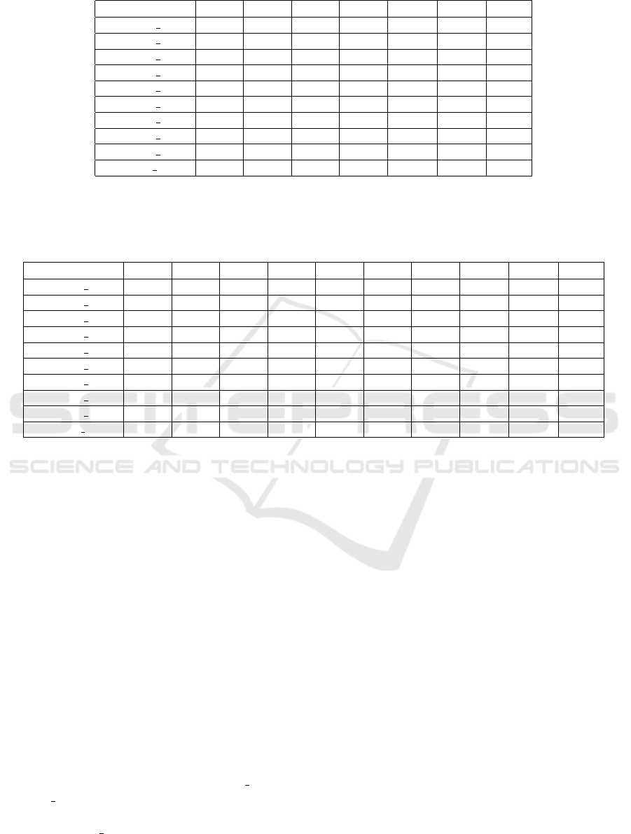
Table 1: Predicted Accuracy and Actual Accuracy of Viterbi Algorithm for a 3 × 3 HMM.

Scenario cos1 cos2 cos3 Mean

Error

Scenario 3(1) 0 0 0 0 100% 100% 0%

Scenario 3(2) 0.133 0.521 0.127 0.261 83% 80% 3%

Scenario 3(3) 0.258 0.258 0.258 0.258 83% 80% 3%

Scenario 3(4) 0.388 0.276 0.266 0.31 79% 76% 3%

Scenario 3(5) 0.313 0.477 0.632 0.474 68% 64% 4%

Scenario 3(6) 0.398 0.405 0.969 0.591 61% 58% 3%

Scenario 3(7) 0.784 0.491 0.849 0.708 52% 52% 0%

Scenario 3(8) 0.956 0.676 0.467 0.699 53% 50% 3%

Scenario 3(9) 0.895 0.830 0.987 0.904 40% 43% 3%

Scenario 3(10) 1 1 1 1 33% 33% 0%

The arithmetic mean of cos1, cos 2, and cos3

The predicted accuracy, given by the formula 1

The actual accuracy of the Viterbi algorithm

Table 2: Predicted and Actual Accuracy Values for the Viterbi Algorithm for a 4 × 4 HMM.

Scenario cos1 cos2 cos3 cos4 cos5 cos6 Mean

Error

Scenario 4(1) 0 0 0 0 0 0 0 100% 100% 0%

Scenario 4(2) 0.043 0.043 0.127 0.127 0.127 0.127 0.099 93% 94% 1%

Scenario 4(3) 0.308 0.308 0.308 0.308 0.308 0.308 0.308 77% 70% 7%

Scenario 4(4) 0.371 0.333 0.254 0.340 0.312 0.446 0.343 74% 68% 6%

Scenario 4(5) 0.449 0.342 0.266 0.528 0.483 0.479 0.424 68% 63% 5%

Scenario 4(6) 0.449 0.582 0.265 0.961 0.446 0.583 0.548 59% 54% 5%

Scenario 4(7) 0.452 0.582 0.268 0.986 0.542 0.580 0.569 57% 54% 3%

Scenario 4(8) 0.427 0.465 0.301 0.873 0.671 0.694 0.572 57% 51% 6%

Scenario 4(9) 0.427 0.526 0.311 0.832 0.768 0.867 0.622 53% 48% 5%

Scenario 4(10) 1 1 1 1 1 1 1 25% 25% 0%

The arithmetic mean of cos1∼cos 6

The predicted accuracy, given by the formula 1

The actual accuracy of the Viterbi algorithm

of emission probabilities. Based on the formula 1 dis-

cussed in Section 3.1, the predicted accuracy is calcu-

lated, then we can get the error between the predicted

accuracy and the actual accuracy.

Similarly, in Table 2 the emission probability has

size 4 × 4, we calculate the cosine similarity for the

six pairs of emission probabilities. Based on the for-

mula 1 discussed in section 3.1, the predicted accu-

racy is calculated, then we can get the error between

predicted accuracy and actual accuracy.

As a quick observation, the cosine similarity of

emission probability dramatically affects the accuracy

of the Viterbi algorithm. When the overall cosine sim-

ilarity is high, the accuracy of the Viterbi algorithm

decreases. On the contrary, the accuracy of the Viterbi

algorithm is higher when the arithmetic mean of co-

sine similarity is smaller.

Consider the two scenarios: Scenario 3(2) and

Scenario 3(3) in Table 1. There is a certain differ-

ence in the cosine similarity of the emission proba-

bility of Scenario 3(2), but their arithmetic means are

the same, and therefore, the predicted accuracy is also

the same.

4.3.1 Error Rate

Combining the results in Table 1 and Table 2, the

range of error is between 0% and 7%. Moreover, we

found the overall error in Table 1 is smaller, which is

about 2%.

5 CONCLUSIONS AND FUTURE

WORK

In this paper, we have attempted to predict the accu-

racy of the well known and well studied the Viterbi

algorithm in simple terms, speciﬁcally in terms of the

cosine similarity of the emission matrix. The experi-

mental results show that the proposed formula for pre-

dicted accuracy matches the observed accuracy very

well.

In this work, we assumed a random transition ma-

trix, but clearly, it can have a signiﬁcant impact on

ICAART 2021 - 13th International Conference on Agents and Artiﬁcial Intelligence

944

the accuracy as well. Just as a quick example, if some

part of the HMM network can never be “reached” due

to the transition probabilities, that part of the HMM

network should have no role in the prediction of the

hidden states. However, this analysis is not covered

in the current paper, and future work can consist of

studying the relationship between transition probabil-

ity and the accuracy of the Viterbi algorithm.

REFERENCES

Blunsom, P. and Cohn, T. (2011). A hierarchical pitman-

yor process hmm for unsupervised part of speech in-

duction. In Proceedings of the 49th Annual Meeting

of the Association for Computational Linguistics: Hu-

man Language Technologies, pages 865–874.

Gales, M. J. (1998). Maximum likelihood linear transfor-

mations for hmm-based speech recognition. Com-

puter speech & language, 12(2):75–98.

Galton, F. (1892). Finger Prints. Macmillan and Company.

all, L., Krogh, A., and Sonnhammer, E. L. (2005). An

hmm posterior decoder for sequence feature predic-

tion that includes homology information. Bioinfor-

matics, 21(suppl 1):i251–i257.

Russell, S. and Norvig, P. (2009). Artiﬁcial Intelligence:

A Modern Approach. Prentice Hall Press, USA, 3rd

edition.

Stamp, M. (2004). A revealing introduction to hidden

markov models. Department of Computer Science San

Jose State University, pages 26–56.

Sung-Hyun, Y., Thapa, K., Kabir, M. H., and Hee-Chan,

L. (2018). Log-viterbi algorithm applied on second-

order hidden markov model for human activity recog-

nition. International Journal of Distributed Sensor

Networks, 14(4):1550147718772541.

Viterbi, A. (1967). Error bounds for convolutional

codes and an asymptotically optimum decoding al-

gorithm. IEEE Transactions on Information Theory,

13(2):260–269.

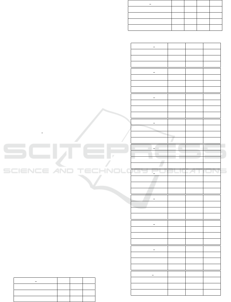
APPENDIX

In appendix, Table 3 represents the transition matrix

of 3×3, Table 4 represents the transition matrix of 4×

4. Table 5 and Table 6 are the corresponding emission

matrices.

Table 3: Transition Matrix 3 × 3.

Scenario 3(1∼10) T1 T2 T3

S1 1/3 1/3 1/3

S2 1/3 1/3 1/3

S3 1/3 1/3 1/3

Table 4: Transition Matrix 4 × 4.

Scenario 4(1∼10) T1 T2 T3 T4

S1 1/4 1/4 1/4 1/4

S2 1/4 1/4 1/4 1/4

S3 1/4 1/4 1/4 1/4

S4 1/4 1/4 1/4 1/4

Table 5: Emission Matrix 3 × 3.

Scenario 3(1) E1 E2 E3

S1 1 0 0

S2 0 1 0

S3 0 0 1

Scenario 3(2) E1 E2 E3

S1 0.99 0.005 0.005

S2 0.1 0.25 0.65

S3 0.1 0.75 0.15

Scenario 3(3) E1 E2 E3

S1 0.8 0.1 0.1

S2 0.1 0.1 0.8

S3 0.1 0.8 0.1

Scenario 3(4) E1 E2 E3

S1 0.8 0.1 0.1

S2 0.1 0.1 0.8

S3 0.2 0.7 0.1

Scenario 3(5) E1 E2 E3

S1 0.8 0 0.2

S2 0.24 0.25 0.51

S3 0.2 0.7 0.1

Scenario 3(6) E1 E2 E3

S1 0.5 0.2 0.3

S2 0.1 0.8 0.1

S3 0.45 0.1 0.45

Scenario 3(7) E1 E2 E3

S1 0.6 0.2 0.2

S2 0.4 0.5 0.1

S3 0.45 0.1 0.45

Scenario 3(8) E1 E2 E3

S1 0.1 0.4 0.5

S2 0.25 0.4 0.35

S3 0.4 0.6 0

Scenario 3(9) E1 E2 E3

S1 0.4 0.2 0.4

S2 0.3 0.4 0.3

S3 0.3 0.5 0.2

Scenario 3(10) E1 E2 E3

S1 0.333 0.333 0.333

S2 0.333 0.333 0.333

S3 0.333 0.333 0.333

Pairwise Cosine Similarity of Emission Probability Matrix as an Indicator of Prediction Accuracy of the Viterbi Algorithm

945

Table 6: Emission Matrix 4 × 4.

Scenario 4(1) E1 E2 E3 E4

S1 1 0 0 0

S2 0 1 0 0

S3 0 0 1 0

S4 0 0 0 1

Scenario 4(2) E1 E2 E3 E4

S1 0.94 0.02 0.02 0.02

S2 0.02 0.94 0.02 0.02

S3 0.02 0.02 0.94 0.02

S4 0.02 0.02 0.02 0.94

Scenario 4(3) E1 E2 E3 E4

S1 0.7 0.1 0.1 0.1

S2 0.1 0.7 0.1 0.1

S3 0.1 0.1 0.7 0.1

S4 0.1 0.1 0.1 0.7

Scenario 4(4) E1 E2 E3 E4

S1 0.7 0.15 0.1 0.05

S2 0.1 0.7 0.1 0.1

S3 0.1 0.1 0.6 0.2

S4 0.1 0.1 0.1 0.7

Scenario 4(5) E1 E2 E3 E4

S1 0.7 0.15 0.1 0.05

S2 0.1 0.5 0.2 0.2

S3 0.1 0.1 0.6 0.2

S4 0.1 0.1 0.1 0.7

Scenario 4(6) E1 E2 E3 E4

S1 0.7 0.15 0.1 0.05

S2 0.1 0.5 0.2 0.2

S3 0.1 0.1 0.05 0.75

S4 0.1 0.1 0.1 0.7

Scenario 4(7) E1 E2 E3 E4

S1 0.7 0.15 0.1 0.05

S2 0.1 0.5 0.2 0.2

S3 0.1 0.1 0.05 0.75

S4 0.1 0.2 0.1 0.6

Scenario 4(8) E1 E2 E3 E4

S1 0.7 0.15 0.1 0.05

S2 0.1 0.5 0.3 0.1

S3 0.1 0.1 0.2 0.4

S4 0.1 0.4 0.1 0.4

Scenario 4(9) E1 E2 E3 E4

S1 0.7 0.15 0.1 0.05

S2 0.1 0.5 0.2 0.2

S3 0.1 0.1 0.2 0.4

S4 0.1 0.4 0.1 0.4

Scenario 4(10) E1 E2 E3 E4

S1 0.25 0.25 0.25 0.25

S2 0.25 0.25 0.25 0.25

S3 0.25 0.25 0.25 0.25

S4 0.25 0.25 0.25 0.25

ICAART 2021 - 13th International Conference on Agents and Artiﬁcial Intelligence

946