
Coupled Active Contours for Clue Cell Segmentation from
Fluorescence Microscopy Images
Yongjian Yu
1
and Jue Wang
2
1
Axon Connected, LLC, Earlysville, VA 22936, U.S.A.
2
Department of Mathematics, Union College, Schenectady, NY 12308, U.S.A.
Keywords: Segmentation, Active Contour, Level Set, Fluorescent Microscopy, Clue Cells.
Abstract: Bacterial vaginosis (BV) increases the risk for preterm birth. Immunofluorescent assay provides accurate
counting of the clue cells. However, the massive data make it challenging to manually interpret. Towards
automatic BV diagnostics, we present a coupled active contour method for segmenting the clue cells using
dual-resolution, dual-channel microscopy. The method is formulated in the level set and parametric
frameworks. A fast search locates potential clue cells in the low-resolution scan. Each cell is then imaged at
high-resolution. The clue cells are segmented and quantified. The efficacy of the method is demonstrated
using clinical data. Our method effectively delineates the boundaries of the cell and its nucleus
simultaneously. It is efficient and practical. The clue cell detection results indicate a high accuracy for BV
diagnosis.
1 INTRODUCTION
Preterm birth is the leading cause of neonatal
mortality and morbidity. Approximately 10% of all
births are preterm. The 2019 United Nations
International Children’s Emergency Fund (UNICEF)
data reported an average rate of 18 deaths per 1,000
live births in 2018 (UNICEF 2019a). Globally, 2.5
million children died in the first month of life in
2018 – approximately 7,000 neonatal deaths every
day. The latest report predicts that 52 million
children under 5 will die between 2019 and 2030
(UNICEF 2019b), 47% of which happen during the
first month. Preterm birth can lead to long-term
medical care requirements and lifelong
developmental disabilities. Just within the United
States, preterm birth results in health care costs of
over $26 billion annually. The financial and
emotional toll to afflicted families is staggering. It is
estimated that up to 50% of all preterm births are the
result of vaginal biome abnormalities (Witkin 2015),
such as bacterial vaginosis (BV), trichomoniasis,
and yeast infections.
Through BV assays using wet mount
microscopy, a physician manually selects and
examines approximately 200 epithelial cells over the
brightfield microscope slide, in order to evaluate the
percentage of the clue cells, which are epithelial
cells covered with bacteria. The process is
subjective, time-consuming, and prone to error due
to debris interference. The sensitive and accurate
immunofluorescence (IF) assay improves the
brightfield microscopic diagnosis of BV. Spectral
features of the clue cells and debris augment the
discrimination. Multi-resolution enables fast cell
locating, closer examination of cell morphology and
bacterial contamination. However, the advanced
instrument generates massive data, making it a
challenge for clinicians to find and identify the clue
cells manually, in particular for point-of-care testing.
It is highly valuable to develop an automated system
for clue cell analysis to quickly and accurately
assess BV.
A clinical sample is shown in Figure 1 at 4X and
40X objectives, respectively. The algorithm needs to
first find epithelial cells using a 4X objective, and
then separates them into clue cells and normal cells
using a 40X objective. The problem of clue cell
segmentation refers to the process of automatically
identifying the cells for characterization and
enumeration. In general, it is desirable to
simultaneously detect the bacteria, nuclei, and cells
of high scale range present in an image and the
associate bacteria and nucleus with each cell.
144
Yu, Y. and Wang, J.
Coupled Active Contours for Clue Cell Segmentation from Fluorescence Microscopy Images.
DOI: 10.5220/0010265301440151
In Proceedings of the 14th International Joint Conference on Biomedical Engineering Systems and Technologies (BIOSTEC 2021) - Volume 2: BIOIMAGING, pages 144-151
ISBN: 978-989-758-490-9
Copyright
c
2021 by SCITEPRESS – Science and Technology Publications, Lda. All rights reserved
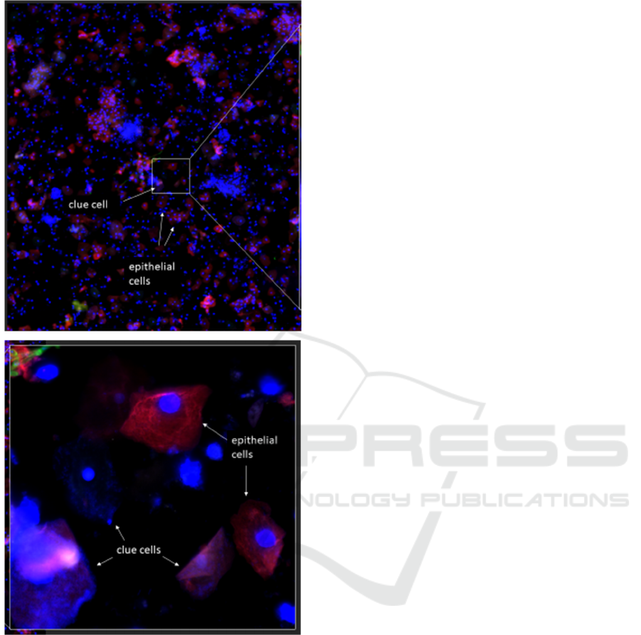
Figure 1: Distinguishing clue cells from normal epithelial
cells. Top image: 4X objective. Bottom zoomed-in image:
40X objective showing clue cells (covered with small blue
dots) and normal cells (little to no blue dots).
In the region-based variational minimization
model, a level set function representation is
introduced together with a contour length or
curvature regularization (Chan and Vese 2001). The
objects are segmented through similarity measures
within the regions. This model is reformulated using
a characteristic function representation with a
length-equivalent total variation regularization
(Zeune et. al. 2017). To achieve multiscale region-
based segmentation, the regularization weight
parameter decreases inversely proportionally to the
steps through a Bregman iteration process. Finally a
spectral analysis is applied to find the cells of
interest.
Watershed transform segmentation has been used
for segmenting partially overlapping objects. The
watershed method is analogue to a landscape
flooded by water. The watersheds are dividing
contours upon which water from different basins
meets, filling catchments corresponding to the local
minima. The method is applied to segment epithelial
cells from bright field microscopy (Tareef et. al.
2018).
We propose two coupled active contour (CAC)
models. The main goal of this work is to present a
multiscale segmentation method combining edge-
region-based active contour methods at high-
resolution with low-resolution watershed
segmentation.
In our work, the vaginal samples are pre-stained
using a pan cytokeratin (CK) cocktail and 46-
diamidino-2-phenylindole (DAPI), the former
labelling the entire cell and the latter for the nucleus
only. The live epithelial cell is our target, thus it
must have a nucleus. An advanced microscope
acquires images at 385-nm and 490-nm channels
using a 4X objective and a 40X objective. The area
of the sample on the slide is about 15 mm by 15 mm,
requiring 25 4X partially overlapped images to scan.
The same area would need 2500 40X images (each
of 2K by 2K pixels, 16-bit/pixel) to cover, which is
prohibitive in time consuming and storage
demanding. Therefore, a 4X fast search over the
whole area followed by a 40X spotlight imaging
balances the cell detection, characterization and
engineering challenges.
Towards a fast, wide-range searching of
epithelial cells, we process the 4X data by applying
adaptive thresholding techniques to the CK-
sensitive, 385-nm band to find the whole cells (CK
blobs for short), and to the 490-nm channel for
masking the nuclear blobs. Any clump of nuclei is
identified by a size threshold and split using a
marker-controlled watershed method. The nuclear
markers are located as the local extended
fluorescence maxima. A clump of cells is identified
by the number of nuclei inside and spilt via the same
watershed controlled by the nuclear markers. A 4X
segmentation of the epithelial cells and associated
nuclei is shown in Figure 2. The epithelial cells are
in red color and the nuclei are blue inside the red.
The isolated darker blue blobs are the white blood
cells.
Coupled Active Contours for Clue Cell Segmentation from Fluorescence Microscopy Images
145
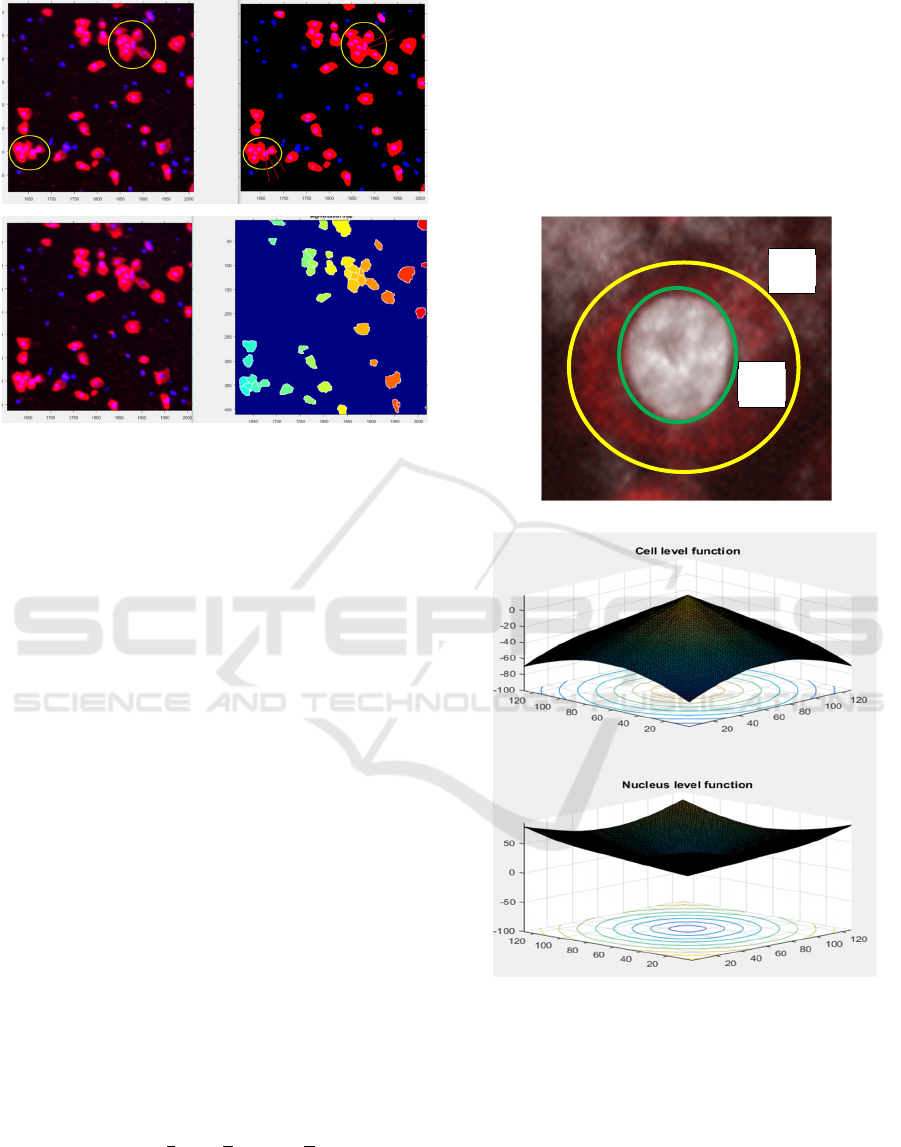
Figure 2: 4X composite image and segmentation of the
epithelial cells and nuclei. The nuclei are the blue blobs
inside the epithelial cells in red.
2 COUPLED ACTIVE CONTOUR
MODELS
2.1 40X Segmentation of Isolated
Epithelial Cell
We describe the first coupled active contour model
for processing the 40X image to delineate the
boundaries of the nucleus and membrane of an
epithelial cell randomly selected from a pool of 4X
segmentation. The goal is to identify whether the
epithelial cell is a clue cell through detection and
enumeration of bad bacteria in the cytoplasm region.
Let 𝑰=
𝐼
𝐼
be a dual-band IF image
(acquired with 40X objective) defined on the domain
Ω, where the superscript T denotes transpose, and
the subscripts indicate the nucleus or cell. Denote 𝑪
⃗
and 𝑪
⃗
a couple of nested closed curves. Let 𝑪
⃗
represent the zero-level set of a signed distance
function 𝜙:Ω → 𝑅, such that 𝑪
⃗
=
{
𝒙|𝜙 = 0
, with
the interior being negative valued. The exterior of 𝑪
⃗
is specified by the regularized Heaviside function
(Chan and Vese 2001),
ℋ
(
𝜙
)
=
1 +
arctan
, (1)
where 𝜖0 is a small regularization parameter. The
interior of 𝑪
⃗
is then defined as ℋ
(
−𝜙
)
.
Likewise, let 𝑪
⃗
represent the zero-level set of a
signed distance function 𝜑: Ω → 𝑅, such that 𝑪
⃗
=
{
𝒙|𝜑 = 0
, with the exterior being negative valued.
Similarly, we specify the interior of 𝑪
⃗
by ℋ
(
−𝜑
)
and the exterior of C
n
as ℋ
(
𝜑
)
. Therefore, the
cytoplasm region is given by ℋ
(
−𝜙𝜑
)
. The
epithelial cell in dual band IF and level set functions
are illustrated in Figure 3.
(a)
(b)
Figure 3: (a) Epithelial cell in dual band IF composite
pseudo-colored image. The green and yellow contours
depict boundaries of the nucleus and membrane,
respectively. The central white region is the Dapi stained
nucleus. The red region between contours is CK-labeled
cytoplasm. (b) Level set functions of the nucleus and
membrane boundaries.
We construct coupled flows on the vectorized
level set
𝜑 𝜙
that continuously attract 𝑪
⃗
toward
the nuclear boundary while simultaneously attracting
𝑪
⃗
𝑪
⃗
BIOIMAGING 2021 - 8th International Conference on Bioimaging
146

𝑪
⃗
toward the cell membrane boundary under the
constraint that the former is completely enclosed by
the latter. We devise the energy functional
𝐸
(
𝜑,𝜙
)
= ℋ
(
−𝜑
)
(
𝐼
(
𝒙
)
−𝑢
)
+
(2)
ℋ
(
−𝜙𝜑
)(
𝐼
(
𝒙
)
−𝑣
)
+ ℋ
(
−𝜙𝜑
)(
𝐼
(
𝒙
)
−𝑢
)
+ ℋ
(
𝜙
)(
𝐼
(𝒙) − 𝑣
)
𝑑𝑎
where 𝒙=
(
𝑥,𝑦
)
,𝑑𝑎 = 𝑑𝑥𝑑𝑦, 𝑢
and 𝑣
represent
the average 𝐼
values of nucleus and cytoplasm,
respectively; 𝑢
and 𝑣
represent the average 𝐼
values of cytoplasm and the background (cell
exterior region), respectively.
To keep both the interior and exterior curves
smooth, we add length regularizations,
𝐸
(
𝜑,𝜙
)
=𝐸
(
𝜑,𝜙
)
+ 𝜆
𝛿
(
𝜑
)|
∇𝜑
|
+𝜆
𝛿
(
𝜙
)|
∇𝜙
|
𝑑𝑎
(3)
where 𝛿
(
𝑧
)
=ℋ
(
𝑧
)
; 𝜆
and 𝜆
are positive
weights for the nucleus and cell contours,
respectively. A smaller weight corresponds to
smaller objects. The goal is to find constrained
minimizers to (3)
min
,
ℋ
(
)
⊆
ℋ
(
)
𝐸
(
𝜑,𝜙
)
(4)
where ℋ
(
−𝜑
)
⊆ℋ
(
−𝜙
)
is the cell-nucleus
enclosure constraint that keeps the computed nuclear
contour from migrating outside the membrane.
If any part of 𝑪
⃗
migrates outside 𝑪
⃗
during
evolution, then the extruding area of that part is
𝐵
(
𝜑,𝜙
)
=
ℋ
(
𝜙
)
ℋ
(
−𝜑
)
𝑑𝒙
. (5)
The enclosure constraint dictates that 𝐵
(
𝜑,𝜙
)
=0 if
the optimal segmentations of the membrane and
nucleus boundaries are obtained. Relaxing the cell-
nucleus enclosure constraint in (4), we approximate
(4) by a non-constrained optimization with enclosure
regularization
min
,
𝐸
(
𝜑,𝜙
)
+𝛾𝐵
(
𝜑,𝜙
)
. (6)
Keeping the channels’ regional statistics
{ 𝑢
,𝑣
,𝑢
,𝑣
} fixed, we derive the associated
Euler-Lagrange equations for 𝜑 and 𝜙, respectively,
and formulate the coupled evolution equations
following the idea of steepest descent,
𝜕𝜑
𝜕𝑡
=𝛿
(
𝜑
)
(
𝐼
(
𝒙
)
−𝑢
)
+
𝜙𝛿
(−𝜙𝜑)
𝛿
(
𝜑
)
((
𝐼
(
𝒙
)
−𝑣
)
+
(
𝐼
(
𝒙
)
−𝑢
)
)
+𝛾
ℋ
(
𝜙
)
+𝜆
div
∇𝜑
|
∇𝜑
|
(7)
𝜕𝜙
𝜕𝑡
=𝛿
(
𝜙
)
−
(
𝐼
(𝒙) − 𝑣
)
+
𝜑𝛿
(
−𝜙𝜑
)
𝛿
(
𝜙
)
((
𝐼
(
𝒙
)
−𝑣
)
+
(
𝐼
(
𝒙
)
−𝑢
)
)
−𝛾ℋ
(
−𝜑
)
+𝜆
div
∇𝜙
|
∇𝜙
|
(8)
The equations are solved under Neumann boundary
conditions.
2.2 Segmentation of Cells in Clutter
Clinical scans contain numerous cell clumps where
multiple cells touch or overlap. The CAC level-set
model will degrade if the epithelial cell picked for
close examination is contacted with or inside a
clump of cells. A second CAC parametric model is
proposed towards algorithmic efficiency and higher
numerical stability.
Define a pair of nuclear and cell segmenting
curves, {𝜌
(
𝜃
)
,𝜉
(
𝜃
)
,𝜃∈
0,2𝜋
, that tend to move
towards their corresponding boundaries
simultaneously to minimize the following energy
functional
𝐸
(
{𝜌,𝜉
)
=
𝛼
2
𝜌
(
𝜃
)
+
𝛽
2
𝜌
(
𝜃
)
+
𝛼
2
𝜉
(
𝜃
)
+
𝛽
2
𝜉
(
𝜃
)
+ℰ
(
𝑹
+𝜌
(
𝜃
)
𝑒̂
)
+ℰ
(
𝑹
+𝜉
(
𝜃
)
𝑒̂
)
+ℰ
𝑹
,𝜌
(
𝜃
)
,𝜉
(
𝜃
)
𝑑𝜃
(9)
Subject to an enclosure constraint: 𝜌
(
𝜃
)
𝜉
(
𝜃
)
,
where 𝛼
and 𝛽
are parameters that weigh elasticity
and rigidity on the curves; 𝑒̂
=𝑒̂
cos𝜃 + 𝑒̂
sin𝜃,
with 𝑒̂
and 𝑒̂
being unit vectors in the x and y
direction, respectively. 𝑹
=
(
𝑥
,𝑦
)
is the position
vector of the origin of the cell polar coordinate
(𝑟,𝜃), illustrated in Figure 4. It coincides with the
centroid of the zoomed-in, pre-computed 4X nucleus
mask of the same cell.
Coupled Active Contours for Clue Cell Segmentation from Fluorescence Microscopy Images
147
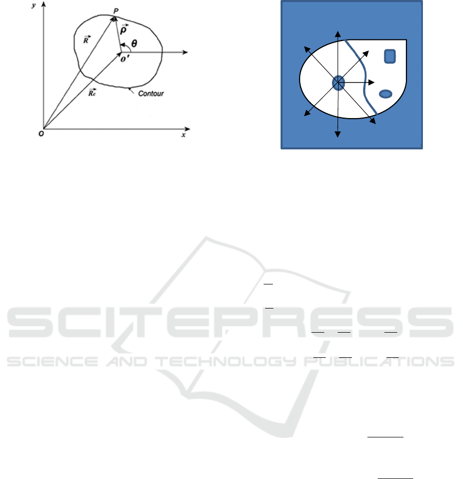
Figure 4: Polar coordinate system representation for
segmenting cells in the clutter environment.
The ℰ
’s are external energy derived from the
image 𝑰=
𝐼
𝐼
and a priori 4X segmentation
such that they take small values near the boundaries
of associated nucleus and cell. ℰ
and ℰ
are driven
by the localized edges in 𝐼
and 𝐼
,
ℰ
(
𝑥,𝑦
)
=−
‖
∇𝐼
(
𝑥,𝑦
)‖
, (10)
ℰ
(
𝑥,𝑦
)
=−
‖
∇𝐼
(
𝑥,𝑦
)‖
. (11)
The ℰ
is region-based. The directional energy along
each radial direction is defined as
ℰ
(
𝜃|𝑹
,𝜌,𝜉
)
=
(
𝐼
(𝑟) −𝑢
)
𝑑𝑟
+
(
𝐼
(𝑟) − 𝑣
)
+
(
𝐼
(𝑟) − 𝑢
)
𝑑𝑟
+
(
𝐼
(𝑟) − 𝑣
(𝜃)
)
𝑑𝑟
(12)
where 𝐼
(𝑟) denotes the profile of 𝐼
(𝑥,𝑦) along the
polar axis r at point 𝑹
with angle 𝜃; 𝑣
(𝜃) denotes
the representative 𝐼
value of the clutter or
background as a function of 𝜃. The 𝑢
, 𝑣
and 𝑢
omni-directional statistics are computed as the
median values using the zoomed-up, registered 4X
mask of the cell. In each direction, 𝑣
is computed as
the median value of 𝐼
in the neighboring cell or in
the background. Figure 5 illustrates how these
statistics are measured with the aid of a 4X mask
and neighborhood adjacency relation. We fix these
values during the contour evolution. The
segmentation is the zoomed-up 4X mask registered
with the 40X image. It is the angle sensitivity that
empowers segmenting cells in a clump environment.
Figure 5: Estimation of the omni-directional statistics
{𝑢
,𝑣
,𝑢
for the nucleus and cell and directional
background statistics 𝑣
. The cell with outward arrows is
the cell under examination. Other touching cells are the
clutters.
We first lift the enclosure constraint in (9) and
derive the Euler-Lagrange equations for the optimal
coupled active contours. The contour evolution
equations are then formulated as follows,
=𝛼
𝜌
(
𝜃
)
−𝛽
𝜌
()
(
𝜃
)
+𝐹
+𝑓
, (13)
=𝛼
𝜉
(
𝜃
)
−𝛽
𝜉
()
(
𝜃
)
+𝐹
+𝑓
, (14)
where −𝐹
=
ℰ
=
ℰ
cos𝜃 +
ℰ
sin𝜃,
−𝐹
=
ℰ
=
ℰ
cos𝜃 +
ℰ
sin𝜃,
which are evaluated on evolving contours 𝜌 and 𝜉 ,
respectively. Using the level set functions 𝜑 and 𝜙
for region representations, we derive the regional
forces as
𝑓
=
(
𝐼
(
𝜌
)
−𝑢
)
+
()
(
)
((
𝐼
(
𝜌
)
−
𝑣
)
+
(
𝐼
(
𝜌
)
−𝑢
)
)
+𝛾ℋ
(
𝜙
)
,
𝑓
=−𝐼
(
𝜉
)
−𝑣
(
𝜃
)
+
(
)
(
)
((
𝐼
(
𝜉
)
−
𝑣
)
+
(
𝐼
(
𝜉
)
−𝑢
)
)
−𝛾ℋ
(
−𝜑
)
,
where the last terms serve as enclosure
regularization forces to ensure nucleus-cell
enclosure similar to (7) and (8).
The first two terms in (13) and (14) comprise the
axially directed internal forces; the last two terms
represent the external forces in the axial direction
driven by local edges and regional statistics. The
internal and external forces compete with each other;
the former resists bending while the latter guides the
contour towards the image edges. The contour of the
40X image is initialized as the boundary of the
BIOIMAGING 2021 - 8th International Conference on Bioimaging
148
corresponding 4X watershed segmentation, and then
10-fold rescaled and post-processed
morphologically. The morphological processing
rectifies the cell shape and size to ensure the
separation of adjacent cells.
2.3 Identification and Characterization
of Clue Cells
Once the epithelial cells are segmented, the clue
cells are identified via bacterial detection over the
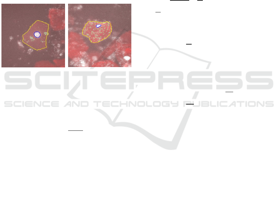
epithelial cytoplasm. In order to detect the tiny
bacteria in the noise, we apply a detail-preserving,
non-local mean filter to suppress the noise. The
bacteria are then found by adaptive thresholding to
the cleaned image, illustrated in Figure 6.
Figure 6: Bacterial detection on epithelial cytoplasm.
We quantify the bacterial contamination of an
epithelial cell using a single metric R, the ratio
between the bacterial area and cytoplasm area. The
likelihood of the clue cell is calculated using the
following expression:
𝑃=Φ
𝑅−𝜇
𝜎
where Φ(𝑥) is a strictly increasing and continuous
function. In this work, Φ takes the form of a
cumulative normal Gaussian distribution function;
the 𝜇 and σ are parameters defining the border
between normal and clue cells. They are determined
under user supervision using a labeled training
dataset.
3 NUMERICAL
IMPLEMENTATION
We devise numerical algorithms for solving the
coupled evolution equations (7) and (8) iteratively.
The level set function 𝜑 and 𝜙 are initialized
through the following steps. We first resize the 4X
image and mask of an epithelial cell of choice to
40X, and then register the zoomed-up 4X image
with the acquired 40X image via cross-correlation.
The registered, zoomed-up 4X mask is used as the
level set initialization. The statistics
{𝑢
,𝑣
,𝑢
,𝑣
are updated during each iteration.
Towards computational efficiency, values of 𝜑 and
𝜙 are updated in their respective narrow bands
around their zero level sets. Re-initialization is
applied using a fast marching scheme (Fatemi and
Sussman 1995). The iteration stops when any
watershed line is crossed by any cell contour. To
achieve numerical stability, image forces are
normalized for each step such that the combined
image forces only update the contour by one pixel.
The contour evolution equation (13) is
discretized as follows,
=
𝜌
⨁
−2𝜌
+𝜌
⊖
−
𝜌
⨁
−2𝜌
⨁
+𝜌
−2𝜌
⨁
−2𝜌
−
𝜌
⊖
+𝜌
−2𝜌
⊖
+𝜌
⊖
+ 𝐹
,
+𝑓
,
,
where Δ𝑡 is the time step and h is the angle
increment, ℎ=
, 𝑁 is the number of angles, 𝜃
=
𝑖ℎ, 𝜌
=𝜌(𝜃
,𝑛∆𝑡), ⊕ and ⊖ are modulo 𝑁
addition and subtraction, respectively.
𝑓
,
=𝑓
(
𝜌
,𝜙
,𝜑
)
,
and
𝐹
,
=−
cos𝜃
ℰ
+
sin𝜃
ℰ
|
,
.
The contour evolution (14) is discretized similarly.
We take 𝑁 to be 64 in our tests. The set of linear
equations is put into a matrix form and solved using
an implicit scheme where Δ𝑡 is set to unity.
4 EXPERIMENTS AND RESULTS
We evaluate the performance of proposed CAC
parametric and CAC level models using a sample of
seven cells. Three cells are isolated intact cells
and the other four belong to two 2-cell
clusters. Example segmentation results are shown in
Figures 7 and 8, along with a comparison to the
multi-pass watershed segmentation (Tareef et. al.
2018). The Dice similarity coefficient and Jaccard
index are used for measuring the segmentation
quality against the expert drawn ground truth. The
Dice similarity coefficient is a spatial overlap index
with values in the range [0,1]. A similarity of 1
means a perfect match in the segmentation. The
Jaccard index calculates the size of intersection of
Coupled Active Contours for Clue Cell Segmentation from Fluorescence Microscopy Images
149
two binary images divided by the size of their union.
This index compares members of two sets for which
are shared and which are distinct. It is in the range
from 0% to 100%, the higher the percentage, the
more similar the two sets. The metrics are listed in
Tables 1 and 2.
To further demonstrate and assess the
performance of our algorithm, we analyze an
example patient sample for BV diagnosis based on
the 20% clue cell diagnostic rule, and compare the
results with clinician detection. From the patient
sample an ensemble of 200 entries were randomly
selected. 48 of 55 clue cells (positive) and 134 of
145 normal epithelial cells (negative) identified by
CAC match the clinician detection. The sensitivity =
0.81, specificity = 0.95, precision = 0.87, and
accuracy = 0.91. The confusion matrix is illustrated
in Table 3. Both the clinician and CAC detection
agree that the patient is BV positive. Our method
segments the cell boundaries very accurately for
80% of the cells. Bacteria clumps and bordering clue
cells result in the false positives. In the case where
the cell images are out of focus, CAC correctly
identifies the cells as non-clue (negative).
The algorithm is implemented in C++ and
integrated with a proprietary digital fluorescence
microscope operated with Intel i9, 8-core processor
and 32 GB RAM in the Windows 10 Pro
environment. The BV scan analysis software
processes a patient sample mounted on a slide. The
imaging pipeline begins after a sample slide is
loaded onto the motorized stage of the microscope.
The system first acquires 25 4X-objective sub-scan
images covering the region of the slide, and
meanwhile searches, in parallel, for all epithelial
cells with the 4X search algorithm, resulting in up to
200 cells randomly distributed for further detailed
analysis. Then, after switching to a 40X objective
and stage movement, it refocuses at each of the
selected 4X cell’s positions, images at 40X of each
cell, and applies the 40X segmentation algorithm to
contour the cell boundary, followed by bacteria
detection, quantification, and clue cell ranking. The
total time of the entire imaging pipeline running in
the microscopic operating system takes less than 10
minutes. The BV processing time is less than half of
that total time. The time for LED exposure, 40X
objective point-wise refocusing, stage movement,
and data transferring from the digital camera to
computer is all included in the 10 minutes.
Our detection algorithm is efficient and practical.
It performs well and demonstrates a high accuracy in
the test-heavy samples.
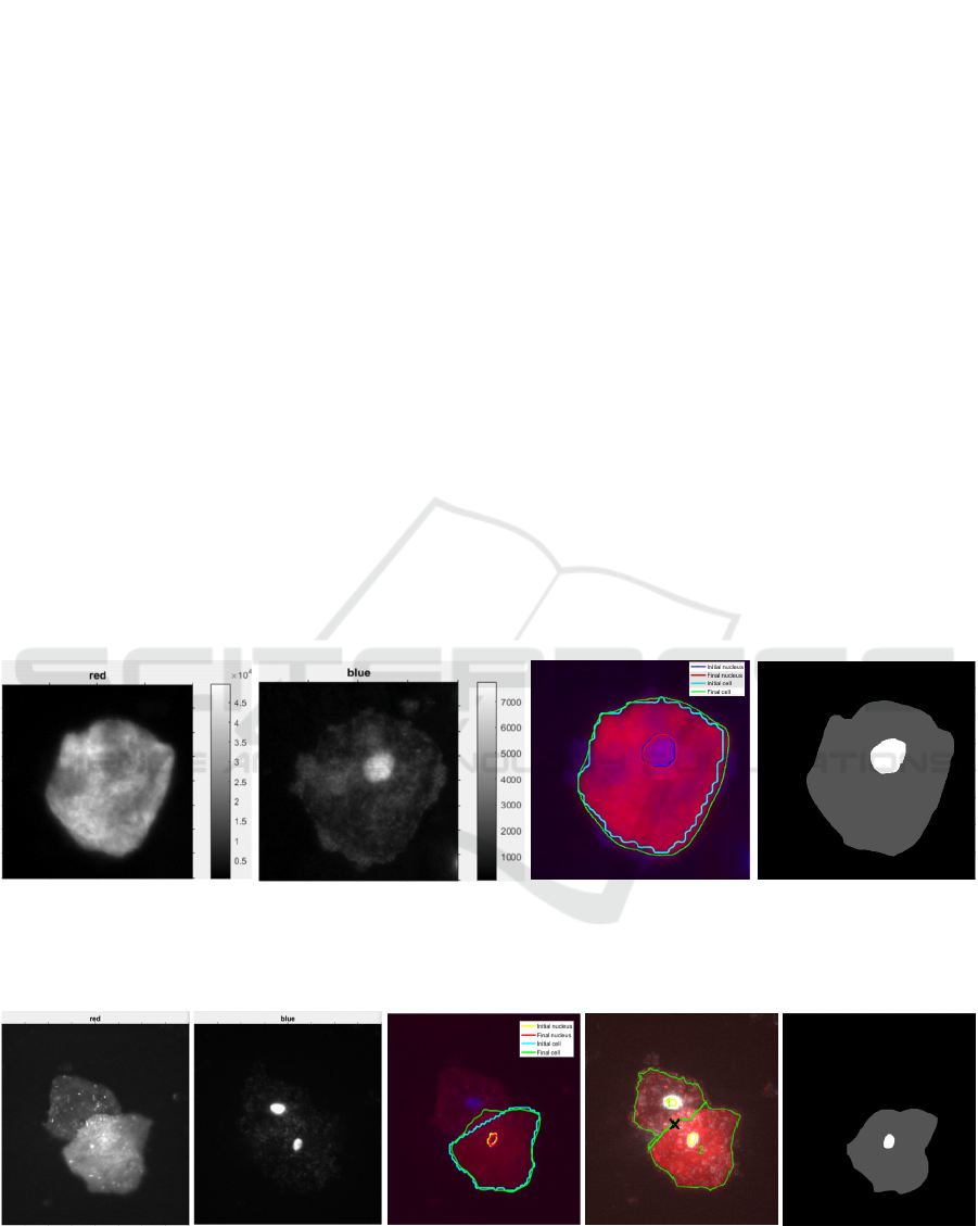
(a) (b) (c) (d)
Figure 7: Segmentation of an isolated epithelial cell. (a) CK channel I
c
. (b) DAPI channel I
n
. (c) CAC level set
segmentation. The nucleus and membrane contours are in red and green, with initialization in blue and cyan, respectively.
(d) Ground truth: nucleus (bright) and cytoplasm (gray).
(a) (b) (c) (d) (e)
Figure 8: Segmentation of partially overlapping epithelial cells. (a) CK channel I
c
. (b) DAPI channel I
n
. (c) CAC parametric
segmentation for the bottom cell. (d) Multi-pass watershed. (e) Ground truth: nucleus (bright) and cytoplasm (gray).
BIOIMAGING 2021 - 8th International Conference on Bioimaging
150

Table 1: Average Dice Index for Nucleus and Cell.
Single cell Overlapped
Nucleus Cell Nucleus Cell
CAC
level set
0.86 0.98 0.87 0.95
CAC
parametric
0.84 0.98 0.82 0.97
Multi-pass
watershed
0.81 0.98 0.87 0.95
Table 2: Average Jaccard Index for Nucleus and Cell.
Single cell Overlapped
Nucleus Cell Nucleus Cell
CAC
level set
0.74 0.96 0.76 0.89
CAC
parametric
0.68 0.96 0.68 0.94
Multi-pass
watershed
0.65 0.95 0.74 0.89
Table 3: Confusion Matrix for CAC Method.
Total = 200
Actual
Positive Negative
Predicted
Positive
True Positive
TP = 48
False Positive
FP = 7
Negative
False Negative
FN = 11
True
Negative
TN = 134
5 CONCLUSIONS
We have developed two coupled active contour
(CAC) models, one with a level set formulation and
the other parametrically, for segmenting the clue
cells and nuclei from the dual-band fluorescence
microscope scans of vaginal samples for bacterial
vaginosis diagnosis. Our models cannot be
categorized simply as a vectorized active contour
method because the channels are treated
independently and the curves evolve cooperatively.
The model is augmented with a coarse-resolution
preprocessing. The imposed enclosure constraint is
tailored to the nested annular shapes. The CAC
method is adaptive for the complex cluttered cell
environment, where the polar model is devised as
coupled parametric snakes that are driven by local
edge forces and long-range regional forces
formulated in the level set representation. While
application-oriented, our effort adds new
contributions to the active contour methodology.
REFERENCES
R. E. Behrman, A.S. Butler (editors), Preterm birth:
causes, consequences, and prevention, Washington,
DC: The National Academies Press, 2007.
T. Brox and J. Weickert, “Level set segmentation with
multiple regions”, IEEE Trans. Image Process., vol.
15, no. 10, pp. 3213-3218, 2006.
T. F. Chan and A. Vese, “Active contours without edges”,
IEEE Trans. Image Process., vol. 10, no. 2, pp. 266-
277, 2001.
E. Fatemi and M. Susman, “An efficient interface
preserving level-set re-distancing algorithm and its
application to interfacial incompressible two-phase
flow”, SIAM J. Sci. Statist Comput., vol. 158, no. 1,
pp. 36-58, 1995.
A. Farr, H. Kiss, M. Hagmann, S. Machal, I. Holzer, V.
Kueronya, P.W. Husslein and L. Petricevic, “Role of
lactobacillus species in the intermediate vaginal flora
in early pregnancy: a retrospective cohort study”,
PLoS One, vol. 10, no. 12, e0144181, 2015.
A. Tareef, Y. Song, H. Huang, D. Feng, M. Chen, Y.
Wang and W. Cai, “Multi-pass fast watershed for
accurate segmentation of overlapping cervical cells”,
IEEE Trans. Med. Imag., vol.37, no.9, pp. 2044-2059,
2018.
UNICEF 2019a, The United Nations International
Children’s Emergency Fund, “Neonatal mortality”,
Sept. 2019. https://data.unicef.org/topic/child-survival
/neonatal-mortality.
UNICEF 2019b, United Nations International Children’s
Emergency Fund, Levels and trends in child mortality,
United Nations Inter-Agency Group for Child
Mortality Estimation (UN IGME), Report 2019.
https://data.unicef.org/resources/levels-and-trends-in-
child-mortality.
S.S. Witkin, “The vaginal microbiome, vaginal anti-
microbial defence mechanisms and the clinical
challenge of reducing infection-related preterm birth”,
BJOG, vol. 122, no. 2, pp. 213-218, 2015.
L. L. Zeune, G. van Dalum, L.W.M.M. Terstappen, S.A.
van Gils and C. Brune, “Multiscale segmentation via
Bregman distances and nonlinear spectral analysis”,
SIAM J. Imag. Sci., vol. 10, no. 1, pp. 111-146, 2017.
Coupled Active Contours for Clue Cell Segmentation from Fluorescence Microscopy Images
151
