
A Decision Guidance System for Optimal Operation of Hybrid Power
Desalination Service Network
Bedor Alyahya and Alexander Brodsky
a
Department of Computer Science, George Mason University Fairfax, VA 22030, U.S.A.
Keywords:
Desalination, Water Management, Optimization, Decision Guidance, Operational Performance, Service
Network.
Abstract:
While modeling and optimization of desalination systems’ operation have been extensively studied, current
approaches are hard-wired to specific designs and performance metrics, without the flexibility to reuse or
extend these models. Bridging this gap, reported in this paper is the development of a formal analytic model
and a decision guidance system for desalination service networks that can be applied to a broad range of
desalination designs and architectures. The model and the system are based on an extensible repository of
atomic component models, initially including models for pumps, renewable energy sources, water and power
storage, and reverse osmosis units. An experimental study is conducted to demonstrate the flexibility of the
model and system, and its scalability to support realistic size problems.
1 INTRODUCTION
The world is facing a great challenge in satisfying in-
creasing water demand. To deal with the challenge,
the United Nations has formed a plan in its 2030
Agenda to ensure availability and sustainable man-
agement of water for all (UN, 2015). In an attempt
to align with the plan requirements, many solutions
have been proposed to meet the increasing demand
for fresh water while minimizing its negative environ-
mental impacts.
The current trend toward solving the shortage
in freshwater is by combining renewable energy
sources with desalination systems. However, renew-
able sources of energy are intermittent in their sup-
ply of electric power. The uncertainty in both de-
mand and, especially, supply of power creates a new
challenge in operating interconnected system com-
ponents to maximize financial, social and environ-
mental benefits. There has been work on optimiz-
ing desalination systems, from a desalination unit
(Ahmed et al., 2019) through hybrid desalination sys-
tem (Mokheimer et al., 2013) to fully integrated wa-
ter and power supply chains (Al-Nory, 2019; Ab-
delshafy et al., 2018). Also, several studies have
examined strategical challenges in combining renew-
able energy with desalination systems. In (Genc¸o
˘
glu
a
https://orcid.org/0000-0003-1694-0913
and Merzi, 2016), the authors focus on strategical de-
cisions in water desalination supply chain by using
mathematical modeling to optimize investment terms.
Al-Nory and El-Beltagy (2015) focuses on minimiz-
ing the interruption of the power supply by select-
ing optimal pumped hydro storage as well as power
storage (e.g., batteries.) Azhar et al. (2017) propose
an efficient desalination system design combined it
with renewable sources to produce water and energy.
Marques et al. (2014) optimize the investment in wa-
ter infrastructures by adapting a flexible water sys-
tem plan using decision trees. However, these models
are either (1) limited in their focus on specific units
or technologies rather than optimizing the desalina-
tion system as a whole, (2) hard-wired to specific de-
signs and objectives which limit its usability in solv-
ing other designs or optimizing other performance
metrics (Mokheimer et al., 2013; Al-Nory, 2019; Al-
Nory and Brodsky, 2014), or (3) focused on long-
term investment in desalination system infrastructures
while making simplifying assumptions on, rather than
accurately modeling the operation of, the underlying
infrastructures over the time horizon (Al Nory and
Graves, 2013). We believe, however, that accurately
modeling the resource flows, such as of power and
water, within and across the system components over
the given operational period can reveal unseen saving
in both operation and investment.
To bridge the gap, we propose an approach that
416
Alyahya, B. and Brodsky, A.
A Decision Guidance System for Optimal Operation of Hybrid Power Desalination Service Network.
DOI: 10.5220/0010265204160424
In Proceedings of the 10th International Conference on Operations Research and Enterprise Systems (ICORES 2021), pages 416-424
ISBN: 978-989-758-485-5
Copyright
c
2021 by SCITEPRESS – Science and Technology Publications, Lda. All rights reserved
Pure Water
Sea Water
Power Storage(s)
RO plant
water
Storage(s)
low
Reservoir(s)
High
Reservoir(s)
Renewable
source(s)
Hydro
generator(s)
Grid
Power Source(s)
Water Desalination System
Sea Water Pure Water
Water under
pressure
Power Line
Compressed
Air
Batteries
Pump
Station
Figure 1: Desalination Service Network.
helps decision makers optimize desalination system
operation over a given operational window (e.g., 72
hours) without the need to hard-wire the model to
a specific desalination design, architecture or perfor-
mance metrics. More specifically, the contributions
of this paper are threefold. First, we develop a formal
Analytic Model (AM) for desalination Service Net-
works (SN) that can be applied to a broad range of
desalination designs and architectures.
Second, we develop an extensible repository of
analytic models for desalination system components,
which initially includes pumps, renewable energy
sources, water and energy storage and Reverse Os-
mosis (RO) plants. Unlike hard-wired models, our
frameworks allows extending model repository with
additional components, and instantiating an arbi-
trary desalination service network, without any other
model modifications.
Third, based on the developed model repository,
we develop a Decision Guidance System (DGS) that
(1) allows desalination system engineers to instanti-
ate their specific desalination design/architecture, (2)
performs iterative optimization over operational time
windows for the selected objective, such as minimiz-
ing CO
2
-adjusted operational cost, while satisfying
the system and demand constraints; and, (3) makes
actionable recommendations to desalination system
operators/control system on precise controls of each
desalination system component for every time inter-
val. The system is based on Decision Guidance An-
alytics Language (DGAL) (Brodsky and Luo, 2015)
and the Decision Guidance Management System ar-
chitecture (Unity DGMS) proposed in (Nachawati
et al., 2017).
Finally, we conduct a preliminary experimental
study to demonstrate the flexibility of the system ap-
plied to four examples of desalination design, and its
scalability to handle realistic size optimization prob-
lems.
The paper is organized as follows. Section 2 il-
lustrates the concept of desalination service network
using an example. Section 3 overviews a high-level
architecture of the developed Desalination Decision
Guidance system and methodology. Section 4 for-
malizes the desalination service network model. Sec-
tion 5 discusses the results of the experimental study.
Finally, Section 6 presents concluding remarks and
briefly outlines directions for future work.
2 DESALINATION SERVICE
NETWORK BY EXAMPLE
The purpose of the Service Network Desalination
Model (SNDM) is to solve a scheduling optimiza-
tion problem for different desalination system designs
and performance metrics. We use a generic struc-
ture called a service network (SN) to allow the model
to handle different designs. The SN, as described in
(Brodsky et al., 2017), is a hierarchy of services that
are connected together to capture the flow of com-
modity over the network. By using a Service Net-
work, we can create different desalination system de-
signs, and through the use of the desalination Ana-
lytical Model AM, we can optimize the performance
metrics of these designs.
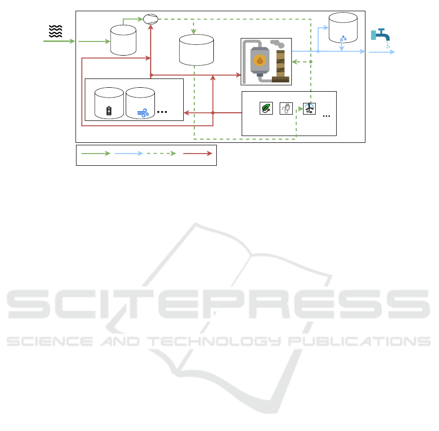
To illustrate this concept, consider an example of
the service network for a hybrid energy system with
Reverse Osmosis (RO) desalination plant system de-
picted in Fig 1. The root of the service hierarchy is
the Water Desalination System. Within it there are
sub-services for a Pump Station, Low Reservoir, High
Reservoir, Power Sources, Power Storage. These ser-
vices are connected together to produce fresh water.
A Decision Guidance System for Optimal Operation of Hybrid Power Desalination Service Network
417

In the figure, each arrow indicates the flow of some re-
source (such as sea water, water under pressure, fresh
water and power) between these services. A com-
posite service, such as Power Sources, contains other
sub-services, such as Renewable Sources and Power
Grid, which are atomic services (i.e., do not have sub-
services.) Both atomic and composite services are op-
tional. Now, we can create many designs by extend-
ing the hierarchy with other sub-services that mimic
the system we intend to represent.
In order for a system to satisfy fresh water de-
mand for a given operational window, it should pro-
duce fresh water by setting the right amount of flows
throughout the system while minimizing the produc-
tion cost and the carbon emissions for a given oper-
ational window. Optimization is based, as described
in Section 4, on an analytic model (AM) which com-
putes metrics such as cost and CO2 emissions, as well
as feasibility constraints, for a given operational win-
dow (e.g., of 72 hours), as a function of operational
controls for each component and time interval (e.g., of
1 hour.) In the model computation, the flows and fea-
sibility have to be aggregated bottom-up, for all inter-
vals, by recursively calling each composite service its’
sub-services starting with the root service until reach-
ing the atomic services at the bottom of the hierarchy.
At that point, the AM uses the type of the atomic ser-
vice to refer to the corresponding atomic AM in the li-
brary of atomic analytical Models (AMs) which then
calculates the flows and feasibility for that atomic ser-
vice. Then, we repeat the same process given the out-
put from the first step but this time we aggregate and
calculate the metrics for the whole periods as well as
some additional constraints described in section 4.
3 DESALINATION DECISION
GUIDANCE SYSTEM
The developed Desalination Decision Guidance Sys-
tem (DGS) (1) allows desalination system engi-
neers to instantiate their specific desalination de-
sign/architecture, (2) performs iterative optimization
over operational time windows for the selected ob-
jective, such as minimizing CO
2
-adjusted operational
cost, while satisfying the system and demand con-
straints; and, (3) makes actionable recommenda-
tions to desalination system operators/control sys-
tem on precise controls of each desalination sys-
tem component for every time interval. The system
is based on Decision Guidance Analytics Language
(DGAL) (Brodsky and Luo, 2015) and the Decision
Guidance Management System (Unity DGMS) pro-
posed in (Nachawati et al., 2017), which in turn is
based on the concept proposed in (Brodsky and Wang,
2008).
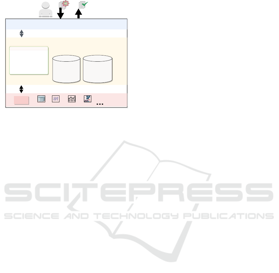
Figure 2 depicts the high-level architecture of De-
salination DGs. The middle layer represent the de-
cision guidance management system that contains
a repository of reusable, modular, and composable
models. Through the Graphical User Interface (GUI),
the user can construct many desalination designs.
Through the analytical engine, the DGMS hides
from the user the complexity in dealing with exter-
nal tools to perform different analytical tasks (such
as optimization, learning and prediction). For ex-
ample, to perform optimization for desalination ser-
vice network, the analytics engines machine generates
a mixed-integer linear programming (MILP) model
from the simulation-like analytic model (formalized
in Section 4), which was written in Python. The in-
put required for DG optimization includes (1) an an-
alytic model, (2) an analytic model input annotated
to indicate which input values serve as decision vari-
ables, and (3) indication of which of the computed
model metrics serves as optimization objective and
constraints.
For desalination plant users, we envision the fol-
lowing workflow for using Desalination DGS:
1. A desalination plant engineer interacts with the
DGS to create an instance of the plant’s design
and architecture.
2. An desalination plant engineer interacts with the
DGS to instantiate additional system parameters,
such as the length of operational window (e.g., 72
hours), and the frequency of re-optimization (e.g.,
at the top of every hour)
3. A plant operator, on a periodic basis, updates the
demand for fresh water. The system performs op-
timization and makes actionable recommendation
on precise controls of every system component,
every operational interval. Some of these con-
trols can automatically actuate the underlying sys-
tem components, whereas some other will be dis-
played to the plant operator, who can approve and
actuate plant controls.
4 FORMALIZATION OF
SERVICE NETWORK
DESALINATION MODEL
4.1 High-level Optimization Problem
The desalination operational optimization is based on
the analytic performance model (AM), which com-
ICORES 2021 - 10th International Conference on Operations Research and Enterprise Systems
418
Input
Output
Decision Guidance Management System
Graphical User Interface
Optimize
Learn
Predict
Simulate
Estimate
...
Analytical Engine
Atomic Models: Composite Models:
Optimization Learning simulationDBMS
Reusable, Extensible, Modular Model Repository
Destination SN
...
Pump
OR
Solar panels
local generator
...
Tools
Figure 2: Desalination Guidance System Architecture.
putes performance metrics, such as cost and carbon
emissions, as well as feasibility constraints, as a func-
tion of fixed and control (decision) parameters of the
desalination service network over the operational time
window. More formally, the analytic performance
model AM is a function:
AM : IN → OU T (1)
The AM forms a valid output instance out ∈ OUT
of performance metrics, such as operational cost or
waste, from a valid input in ∈ IN of fixed and con-
trolled operational parameters.
Then, the desalination optimization problem is:
min
in ∈ IN
ob j(AM(in))
s.t. C(AM(in))
(2)
where
• Ob j : OUT → R is an objective function, which
gives the real objective value in R given a valid
output instance of the AM.
• C : OUT → {T, F} is a constraint function C,
which gives True or False given a valid output in-
stance of the AM.
In contrast of hardwired models, we describe the
objective and constraints as a function of analytical
model AM output. By doing that we loosening the
tightly connected model, so that same AM can be
used to formulate multiple desalination optimization
problems using different system designs and objective
functions.
In the following, we will use the following nota-
tion for a set of key-value pairs:
m ={key
1
: value
1
, key
2
: value
2
,
. . . key
n
: value
n
}
(3)
where the keys are unique identifiers. Note that this
set represents a mapping
m : {key
1
, . . . , key
n
} −→ ∪
n
i=1
D
i
from the set of keys to union of the domains so
that m(key
i
) ∈ D
i
for all i = 1, . . . , n. We will use
the notation keys(m) = {key
1
, . . . , key
n
} to denote
the set of all keys associated with the set m of key-
value pairs.
Now using the above notations we can describe all
of the components above; starting with a valid ser-
vice network desalination model output instance out
in section 4.2, followed by the input instance in in sec-
tion 4.3, and finally, we describe the analytic model
which is a function that computes an output instance
from the input instance.
4.2 Service Network Desalination
Instance: The Model Output
A valid SN desalination output instance out is a set of
key:value pairs:
{config : h config parametersi
rootServiceID : root service id,
services : h set of servicesi,
constraints : ”True”or”False”,
metrics : h set of metricsi}
(4)
where:
• config value is a set of:
{operationalInterval : value,
operationalWindow :w}
where config value defines the time horizon us-
ing the operationalInterval string that repre-
sents the unit of time in which the system oper-
ates (e.g, hour). The operationalWindow (w)
represents the number of intervals, so that op-
erational decisions can be made over these in-
tervals.
• rootServiceID: is the id of a service in services
designated as a root service.
• Services: is a set optional key:value pairs of the
form:
A Decision Guidance System for Optimal Operation of Hybrid Power Desalination Service Network
419

{powerService :{energyContracts : service
1
,
renewableEnergy : service
2
,
other : service
3
},
lowReservoirs :service
4
,
powerStorage :service
5
,
pumpStation :service
6
,
highReservoirs :service
7
,
desalinationPlant :service
8
,
waterStorage :service
9
}
(5)
where each key represent service id which
uniquely identifies that service and each
service
i
∈ {service
1
. . . service
9
} is either a
composite or an atomic service. As each com-
posite service, such as powerService, contains
at least one subservice, it includes the IDs of
these services under subService. So, each com-
posite service has the following form:
{type : ”composite”,
inFlow :{inF
1
: hf-value i,
inF
2
: hf-value i, . . . },
outFlow :{OutF
1
: hf-value i,
OutF
2
: hf-value i, . . . },
metrics :{cost : hm-value i,
CO
2
: hm-value i, . . . },
constraints :”True”or”False”,
subServices :{set of service ids }}
(6)
where each inFlow and outFlow contains a set
of f
i
and h f-value i pairs that represent the
flows going in and out each service. The form
of each hf-valuei can be express as follow:
{ qty: [num
1
. . . num
w
],
total: numeric value}
where the qty is a sequence that shows the
quantities of flow at each operational inter-
val while the total shows the total flow for
the whole operational window.
In the same manner, the metrics value contains
as set of metrics (such as cost or CO
2
) with
their corresponding hm −valuei in the form of:
{perInt: [num
1
. . . num
w
],
total : numeric value}}
(7)
where the perInt is a sequence that shows
the metric per interval while the total
shows the summation for all intervals.
The constraints value indicates whether the
service satisfies its constraints.
• The metrics shows the metrics for the rootService.
• The constraints indicates whether all the con-
straints of the rootservice are satisfied.
The atomic service has the similar form except that:
• There is no subServices key:value pair.
• The type refers to one of the atomic analytical
model in the library.
• Additional set of key:value pair:
onFlag : [Boolean
1
, . . . ,Boolean
w
]
where each boolean value in the list indicate if the
service is running ”1” or not ”0” at each interval
of the operational window (w).
• An optional set of key value pair:
typeSpecific:{ set of key:value pairs }
where typeSpecific value represents, using a
key:value pairs , the parameters that are needed
by the atomic analytic model type to calculate its
metrics and constraints.
• An optional set of key:value pairs:
state : {st
1
: [num
1
. . . num
w
],
st
2
: [num
1
. . . num
w
], . . . }
where the set keys (state) represent the tem-
poral elements inside the service. So, each
st
i
, i maps to a list of numeric values that cap-
ture the state of the service in each interval.
In the next section, we describe a valid input model
needed to compute the output instance.
4.3 Service Network Desalination
Instance: The Model Input
The model input (in) follow the same structure as the
output, but with some modification:
• No metrics and constraints objects.
• Instead of having a list to describe qty for each
flow in the composite service, we replace it with a
list of lower bound (LB).
• For an atomic service:
– Instead of having a list to depict the state, we
replace it with a single value that depicts the
state at the beginning of the operational win-
dow:
state : {st
1
: num
initial
,
st
2
: num
initial
, . . . }
ICORES 2021 - 10th International Conference on Operations Research and Enterprise Systems
420

4.4 Analytic Model (AM)
To describe how analytical model forms the valid out-
put (out) from a valid input (in), we indicate how the
differences between the out (in form 4) and the in are
computed:
let
x = out(rootServiceID) = in(rootServiceID)
then
out(constraints) = out(services)(x)(constraints)
out(metrics) = out(services)(x)(metrics)
out(services) =
[
id∈ID
mOut
opOut
in(services)(id)
Below, we describe how the (opOut) and (mOut)
functions construct the out(services) form from the
input composite and atomic services in(services). In
section 4.4.1, we show how the operationOut (opOut)
calculates out(services) without the metrics. Then,
the result is used, by mertricOut (mOut), to calculate
the metrics in section 4.4.2.
4.4.1 operationOut (opOut)
In this section, we show how the operationOut
(opOut) calculates the inFLow and outFlow quanti-
ties over the operational window as well as some flow
constraints.
The composite service: As in form 6, for every com-
posite service the quantity (qty) of every inFlow and
outFlow is expressed recursively as:
let
SU B = cs(subService)
qtyIn(id, x, y) =
out(services)(id)(inFlow)( f
x
)(qty)[y]
qtyOut(id, x, y) =
out(services)(id)(outFlow)( f
x
)(qty)[y]
then
∀cs ∈ CS, i ∈ keys(inFlow),
j ∈ keys(outFlow), k ∈ {1, . . . , w}
cs(inFlow)( f
i
)(qty)[k] =
∑
sub∈SUB
qtyIn(sub, i, k) − qtyOut(sub, j, k)
cs(outFlow)( f
j
)(qty)[k] =
∑
sub∈SUB
qtyOut(sub, j, k) − qtyIn(sub, i, k)
Therefore, the (total) for every inFlow and outFlow
are:
cs(inFlow)( f
i
)(total) =
w
∑
k=1
services(cs)(inFlow)( f
i
)(qty)[k]
cs(outFLow)( f
j
)(total) =
w
∑
k=1
services(cs)(outFlow)( f
j
)(qty)[k]
Also, for every composite service cs ∈ CS, the
(constraints) expressed as a conjunction of demand-
Constraint(cs), boundConstraint(cs), and subService-
Constraints(cs). Each constraint is expressed recur-
sively as follows:
let SUB = cs(subService)
inKeys(id) = keys(id(inFlow))
outKeys(id) = keys(id(outFlow))
• domandConstraint(cs) ≡
∀sub ∈ SUB, k ∈ {1, . . . , w}
∀i ∈
n
[outKeys(sub)∪ inKeys(sub)]
− [inKeys(cs)∪ outKeys(cs)]
o
qtyIn(sub, i, k) ≥ qtyOut(sub, i, k)
• boundConstraint(cs) ≡
∀i ∈{outKeys(sub)∪ inKeys(sub)}, k ∈ {1 . . . w}
in(cs)(services)(inFlow)(i)(LB)[k]
≥ qtyIn(cs, i, k)
• subServiceConstraints(cs) ≡
∀sub ∈SUB
sub(constraints)
The atomic service (as): For every atomic service
the quantity (qty) of every inFlow and outFlow is cal-
culated by calling the analytical model of its type
(see appendix). Additionally, every atomic con-
straints is expressed as a conjunction of bound Con-
straint, on Flag Constraint. The boundConstraint(as)
is expressed as in the composite service boundCon-
straint(cs), while onFlagConstraint(as) is expressed as
follows:
boundConstraint(as) ≡
∀i ∈ {outKeys(as) ∪ inKeys(as)}, k ∈ {1, . . . , w}
as(onFlog) = 0
→ qtyOut(as, i, k)
A Decision Guidance System for Optimal Operation of Hybrid Power Desalination Service Network
421

Table 1: The optimization time and objective value for the four desalination designs.
Design High
Reservoir
Hydro
generator
Power
Storage
Water
Storage
CPU
time
(s)
Objective
Value
Peak
demand
bound
(k)
Average
power
consump-
tion (KW)
A Yes Yes Yes Yes 3.4 426.54 44.5 9.43
B No No Yes Yes 1.52 472.51 41.71 9.43
C Yes No No No 0.46 436.42 21.00 11.23
D No No No Yes 0.84 472.51 41.71 9.43
The state(as,i) for ∀s ∈ AS and ∀k ∈ {1, . . . , w} is ex-
pressed as:
state(as, i) =
newState(as, k, state(as, k − 1)) , k > 1
as(state) , k = 1
where newState is a function that returns the new state
from a given state for a service with id ∈ AS, and in-
terval i ∈ {1, . . . , w}. Further, the atomic analytical
model updates the serviceSpecific key:value pairs by
adding some information that are needed later on to
calculate the metrics which need larger intervals. For
example, the desalination system operate per hour,
while calculating some metrics like the cost for ener-
gyContract need the knowledge of average consump-
tion for the last two months.
4.4.2 metricOut (mOut)
In this section, we show how the metricOut (mOut)
calculates the metrics over the operational window as
in form 7.
The composite service: For every composite service
every metric (such as cost and CO
2
) are expressed re-
cursively as:
let
mIn(id) = opOut(in(services)(id))
mPerInt(id, x) =
mOut(mIn(id)(metrics)(cost)(perInt)[x])
mTotal(id) =
mOut(mIn(id)(metrics)(cost)(total))
then
∀cs ∈ CS, k ∈ {1, . . . , w}
mPerIn(cs, k) =
∑
sub∈SUB
mPerIn(sub, k)
mTotal(cs) =
∑
sub∈SUB
mTotal(sub)
The atomic service (as): The metrics and constraints
for the atomic services are calculated by calling the
analytical model of its type. Due to page limitation
we omit the formalization of the atomic analytic mod-
els(AMs). More can be found in (Bedor Alyahya,
2020).
5 EXPERIMENTATION
In this section, we show how the proposed desali-
nation AM can support diverse desalination systems.
We run an experimentation that aim to asses the capa-
bility of the model in solving realistic problems using
a machine with a 1.8 GHz Intel Core i5 processor and
8 GB of DDR3 memory executed at 1600 MHz. We
used CPLEX 12 as an optimization tool. We imple-
ment the system using the architecture proposed in
section 3. Then, we create a design that includes low
reservoir, pump, RO plant and power source which
in turn includes renewable source (solar panels) and
the grid. We assume a time horizon of 24 hours and
generate a random supply of renewable energy source
(solar panels), that follow the normal bell shape curve
during the first 12 hours and 0 otherwise. We also use
a power contract agreement which charges extra fee
over its fixed fee using the following formula:
Extra = (k − Avg) ∗ r (8)
where Avg is the average of power consumption over
the time horizon, k is the peak demand bound and r is
the rate of extra kilowatt per hour.
Table 1 shows four different architectures (A, B,
C, D). In architecture A, we add the high reservoir
connected with hydro generator and power and wa-
ter storage to produce the variable demand. In archi-
tecture B, we add power and water storage. while in
architecture C, we only add the high reservoir and in
architecture D we did not add any extra component.
We then specify for each component we added its type
specific parameter (like the maximum capacity for the
water storage). Then, we optimize the the flows of
power and water as well as the peak demand bound
against the following objective function:
Total cost of operation + 0.2 * Total carbon emission
ICORES 2021 - 10th International Conference on Operations Research and Enterprise Systems
422

Table 1 shows the objective values for the four de-
signs. These architectures use different storage tech-
nologies to store excess supplies during intervals of
low demand to satisfy the fluctuations in demand. We
can see that architecture A and C achieve better re-
sults than C and D under the same input assumption.
These comparison can lead to useful insight in know-
ing which component can contribute to the system the
most.
For the purposes of evaluating the model in solv-
ing realistic size problems, we generate four differ-
ent instances from architecture A by varying two di-
mensions:(1) The number of atomic services (AS)
and (2) The number of intervals in the time horizon
(w). Table 2 shows the number of atomic services,
the number of intervals and the time it take the solver
to solve each instance. We can see that when we set
the time horizon (w) to 24 hour, we reach the optimal
solution in 16 seconds and 3 minutes when the num-
ber of atomic services are 78 and 306, respectively.
Whereas, when we use 168 intervals we converge to
near optimal solution within 0.43% gap in 25 seconds
and 1.29% gap in 45 seconds when the number of
atomic services are 42 and 78, respectively. As an
initial step, the solution time to optimality is practical
to operate on an interval (e.g., 1 hour).
Table 2: Shows different variation of problem sizes.
Intervals
(w)
Atomic
Services
(AS)
Gap
(%)
Time
(s)
24 78 0 16
24 306 0 183
168 42 0.03 105
168 78 0.03 693
6 CONCLUSIONS AND FUTURE
WORK
We reported on the development of a formal ana-
lytic model and a decision guidance system for de-
salination service networks that can be applied to a
broad range of desalination designs and architectures.
The model and the system are based on an extensible
repository of atomic component models, initially in-
cluding models for pumps, renewable energy sources,
water and power storage, and reverse osmosis units.
We conducted an experimental study to demonstrate
the applicability of the model and the system to a
range of desalination designs, using four examples,
and the scalability of the solution to realistic size
problem. As future work, we plan to expand the ex-
perimentation to study a realistic water supply chain
using our proposed model. Additionally, we plan to
develop a modular investment model based on the ac-
curate operational model developed in this paper.
REFERENCES
Abdelshafy, A. M., Hassan, H., and Jurasz, J. (2018). Op-
timal design of a grid-connected desalination plant
powered by renewable energy resources using a hy-
brid pso–gwo approach. Energy Conversion and Man-
agement, 173:331–347.
Ahmed, F. E., Hashaikeh, R., Diabat, A., and Hilal, N.
(2019). Mathematical and optimization modelling in
desalination: State-of-the-art and future direction. De-
salination, 469:114092.
Al-Nory, M. (2019). Optimal decision guidance for the
electricity supply chain integration with renewable en-
ergy: Aligning smart cities research with sustainable
development goals. IEEE Access, PP:1–1.
Al Nory, M. and Graves, S. (2013). Water desalination sup-
ply chain modeling and optimization.
Al-Nory, M. T. and Brodsky, A. (2014). Towards optimal
decision guidance for smart grids with integrated re-
newable generation and water desalination. In 2014
IEEE 26th International Conference on Tools with Ar-
tificial Intelligence, pages 512–519.
Al-Nory, M. T. and El-Beltagy, M. (2015). Optimal selec-
tion of energy storage systems. In 2015 Saudi Arabia
Smart Grid (SASG), pages 1–6.
Azhar, M. S., Rizvi, G., and Dincer, I. (2017). Integration of
renewable energy based multigeneration system with
desalination. Desalination, 404:72 – 78.
Bedor Alyahya, A. B. (2020). A decision guidance sys-
tem for optimal operation of hybrid power desalina-
tion service network. Technical Report GMU-CS-TR-
2020-3, Department of Computer Science, George
Mason University, 4400 University Drive MSN 4A5,
Fairfax, VA 22030-4444 USA.
Brodsky, A., Krishnamoorthy, M., Nachawati, M. O., Bern-
stein, W. Z., and Menasc
´
e, D. A. (2017). Manufactur-
ing and contract service networks: Composition, op-
timization and tradeoff analysis based on a reusable
repository of performance models. In 2017 IEEE In-
ternational Conference on Big Data (Big Data), pages
1716–1725.
Brodsky, A. and Luo, J. (2015). Decision guidance analyt-
ics language (dgal). In Proceedings of the 17th Inter-
national Conference on Enterprise Information Sys-
tems - Volume 1, ICEIS 2015, pages 67–78, Portugal.
SCITEPRESS - Science and Technology Publications,
Lda.
Brodsky, A. and Wang, X. S. (2008). Decision-guidance
management systems (dgms): Seamless integration
of data acquisition, learning, prediction and optimiza-
tion. In Proceedings of the 41st annual Hawaii inter-
national conference on system sciences (HICSS 2008),
pages 71–71. IEEE.
A Decision Guidance System for Optimal Operation of Hybrid Power Desalination Service Network
423

Genc¸o
˘
glu, G. and Merzi, N. (2016). Trading-off constraints
in the pump scheduling optimization of water distribu-
tion networks. Journal of Urban and Environmental
Engineering, 10(1):135–143.
Marques, J., Cunha, M., and Savi
´
c, D. (2014). Decision
support for optimal design of water distribution net-
works: A real options approach. Procedia Engineer-
ing, 70:1074 – 1083. 12th International Conference
on Computing and Control for the Water Industry,
CCWI2013.
Mokheimer, E. M., Sahin, A. Z., Al-Sharafi, A., and Ali,
A. I. (2013). Modeling and optimization of hybrid
wind–solar-powered reverse osmosis water desalina-
tion system in saudi arabia. Energy Conversion and
Management, 75:86 – 97.
Nachawati, M. O., Brodsky, A., and Luo, J. (2017). Unity
decision guidance management system: Analytics en-
gine and reusable model repository. In ICEIS (1),
pages 312–323.
UN (2015). Transforming our world : the 2030 agenda for
sustainable development : resolution /. page 35 p. Is-
sued in GAOR, 70th sess., Suppl. no. 49.
ICORES 2021 - 10th International Conference on Operations Research and Enterprise Systems
424
