Weakly Supervised Gleason Grading of Prostate Cancer Slides using
Graph Neural Network
Nan Jiang
1
, Yaqing Hou
1,∗
, Dongsheng Zhou
2
, Pengfei Wang
1
, Jianxin Zhang
3
and Qiang Zhang
1,∗
1
School of Computer Science and Technology, Dalian University of Technology, Dalian 116024, China
2
Key Laboratory of Advanced Design and Intelligent Computing, Ministry of Education, Dalian University,
Dalian 116622, China
3
School of Computer Science and Engineering, Dalian Minzu University, Dalian 116600, China
Keywords:
Prostate Cancer, Gleason Grading, Graph Neural Network, Weakly Supervised.
Abstract:
Gleason grading of histopathology slides has been the “gold standard” for diagnosis, treatment and prognosis
of prostate cancer. For the heterogenous Gleason score 7, patients with Gleason score 3+4 and 4+3 show a
significant statistical difference in cancer recurrence and survival outcomes. Considering patients with Gleason
score 7 reach up to 40% among all prostate cancers diagnosed, the question of choosing appropriate treatment
and management strategy for these people is of utmost importance. In this paper, we present a Graph Neural
Network (GNN) based weakly supervised framework for the classification of Gleason score 7. First, we
construct the slides as graphs to capture both local relations among patches and global topological information
of the whole slides. Then GNN based models are trained for the classification of heterogeneous Gleason
score 7. According to the results, our approach obtains the best performance among existing works, with
an accuracy of 79.5% on TCGA dataset. The experimental results thus demonstrate the significance of our
proposed method in performing the Gleason grading task.
1 INTRODUCTION
Prostate cancer is one of the most common cancers,
seriously affecting around 1 in 9 men all over the
world (Moch et al., 2016). Gleason grading system
has been recognized as the most powerful indicator
for estimating the aggressiveness of prostate cancer,
which is of great significance for instructing its risk
stratification and determining treatment. Specifically,
Gleason score (GS) is defined by a sum of the primary
and secondary patterns present in the tumor area with
the range of 2 to 10. Each pattern is assigned with
a score ranging from 1 (G1) to 5 (G5), that higher
scores indicate more aggressive cancer and poorly dif-
ferentiated glands. In current clinical practice, the
lowest GS assigned is GS 6 (G3 + G3) (Epstein and
Jonathan, 2018), since assignment of GS 2 to 5 have
poor reproducibility and low correlation with radi-
cal prostatectomy grade (Zareba et al., 2010) (Epstein
et al., 2015).
Conventionally, the assessment of GS is carried
out manually by well trained pathologists, which is
time-consuming and suffers from very high inter-
observer variability. In recent years, there is growing
∗
Yaqing Hou and Qiang Zhang are the corresponding au-
thors of this article.
interest in computer-aided automatic Gleason grad-
ing methods based on deep learning techniques, es-
pecially Convolutional Neural Network (CNN). Ex-
isting researches can be roughly categorized into su-
pervised methods (Arvaniti et al., 2018) (Ren et al.,
2018) and weakly supervised methods (del Toro et al.,
2017) (Arvaniti et al., 2018) (Xu et al., 2018) (Wang
et al., 2019) (Pinckaers et al., 2020). However, most
of them have focused on the classification of homo-
geneous tumor regions with only one single Glea-
son pattern (i.e., G3 ,G4 or G5) (Khurd et al., 2010)
(Kallen et al., 2016) (Nagpal et al., 2018) (Pinckaers
et al., 2020) (Wang et al., 2018), or high grades (i.e.,
GS ¿= 8) versus low grades (i.e., GS ¡= 7) (del Toro
et al., 2017) (Ren et al., 2018) (Xu et al., 2018) (Wang
et al., 2019), which are of limited help for clinical di-
agnosis.
In this paper, we mainly focus on the classification
of heterogeneous GS 7 (e.g., G3 + G4 and G4 + G3).
Studies show that GS 7 should be delineated into dif-
ferent prognostic groups since patients with G3 + G4
and G4 + G3 show a significant statistical difference
in cancer recurrence and survival outcomes (Hochre-
iter and Schmidhuber, 1997). Comparing to G3 + G4,
the gland structures in G4 + G3 are poorly differenti-
ated (Epstein et al., 2016). Considering patients with
426
Jiang, N., Hou, Y., Zhou, D., Wang, P., Zhang, J. and Zhang, Q.
Weakly Supervised Gleason Grading of Prostate Cancer Slides using Graph Neural Network.
DOI: 10.5220/0010264804260434
In Proceedings of the 10th International Conference on Pattern Recognition Applications and Methods (ICPRAM 2021), pages 426-434
ISBN: 978-989-758-486-2
Copyright
c
 2021 by SCITEPRESS – Science and Technology Publications, Lda. All rights reserved

GS 7 reach up to 40% among all prostate cancers di-
agnosed (Siegel et al., 2017), the question of choos-
ing appropriate treatment and management strategy
for these people is of utmost importance.
Recently, several studies have been carried out
on the analysis of heterogeneous GS 7. For exam-
ple, (Zhou et al., 2017) proposed an automatic Glea-
son grading method for heterogeneous GS 7. Their
pipeline consists of gland region segmentation by
K-means clustering, color decomposition, and CNN
based classification. (Li et al., 2019) proposed a
two-stage attention based Multiple Instance Learn-
ing (MIL) model that can classify the prostate can-
cer slides into benign, low-grade (i.e., G3 + G3 or
G3 + G4) and high grade (i.e., G4 + G3 or higher).
Both approaches mentioned above are not sufficiently
context-aware and do not capture the correlations
among patches that are predictive of Gleason grad-
ing. (Jian et al., 2018) developed a survival analy-
sis model, further exploring the prognosis of prostate
cancer patients that are graded with G3 + G4 and
G4 + G3. Specifically, they used a CNN based long
short-term memory (LSTM) (Hochreiter and Schmid-
huber, 1997) method to model the spatial relationship
of patches extracted from one slide. However, LSTM
model works in a sequential way, which is not capable
of describing one to many correlations among patches
correctly.
To alleviate the deficiencies, we introduce Graph
Neural Network (GNN), which is an emerging tech-
nology for graph data analyzing, into the Gleason
grading task. In particular, with the introduction of
convolution operator on the basis of GNN, Graph
Convolutional Network (GCN) has a strong ability
of modeling the global information and dependencies
among graph nodes. It updates each node embed-
ding by aggregating the information come from multi-
layer neighborhoods. Then the updated node repre-
sentations are used to complete subsequent tasks (Wu
et al., 2019). (Wang et al., 2019) came up with a GCN
based automatic Gleason grading method that assigns
prostate cancer tissue micro-arrays (TMA) with GS
=6 or GS ¿= 7. Their model can capture the dis-
tribution and spatial relations of cells by modeling
TMAs as cell-graphs through learning nucei features
as nodes. However, the cell-graph is not capable of
modeling the gland structures, which is of great im-
portance in the classification of GS 7. In our work,
for the sake of capturing both gland features and re-
lations among patches, we crop the prostate cancer
slides into small patches to model patch-graphs.
In this paper, we present a GNN based weakly
supervised Gleason grading method, which models
the prostate cancer slides as graphs with patch-level
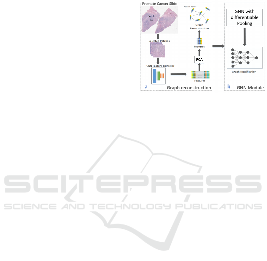
Figure 1: Overview of the GNN based Gleason grading
workflow. a. Graph reconstruction module. b. GNN mod-
ule.
features and introduces two edge construction mech-
anisms. The patch–level feature extractor is trained
on pure slides (GS 3+3 and GS 4+4) to further pro-
mote the accuracy of classification. Our GNN based
model has the inherent ability to accurately capture
both local relations among patches and global topo-
logical information of the tumor area.
The main contributions of this work can be sum-
marized as follows:
• We focus on the classification of heterogeneous
GS 7 that very few researches have studied. We
propose a GNN based weakly supervised method
without relying on the patch-level annotations and
non-tumor slides. To the best of our knowledge,
we are the first to introduce GNN mechanism into
heterogeneous GS 7 classification task.
• We conducted experiments on cancer genome
atlas (TCGA), which is one of the most fa-
mous databases for cancer research. Our model
achieves an accuracy of 79.5% in differentiating
G3 + G4 with G4 + G3, which is superior to state-
of-the-art result.
The rest of this paper is organized as follows. We
first review some related works about automatic Glea-
son grading techniques in Sec. 2. Next, in Sec. 3,
we describe the pipeline of our proposed GNN based
model. Implementation details of the experiments and
final results with analysis are shown in Sec. 4. Fi-
nally, conclusion is present in Sec. 5.
2 RELATED WORK
Existing automatic Gleason grading methods can be
roughly divided into supervised methods and weakly
supervised methods.
Weakly Supervised Gleason Grading of Prostate Cancer Slides using Graph Neural Network
427

2.1 Supervised Gleason Grading
At an earlier stage of computer aided Gleason grad-
ing, (Khurd et al., 2010) assign GS to prostate cancer
slides by classifying texture, which is characterized
by clustering the filter responses extracted from ev-
ery pixel. With the revolution of Convolutional Neu-
ral Networks (CNNs), many researchers train CNN
based classifiers with sufficient fine-grained labels
that manually annotated by pathologists. Several
prevalent CNN models, such as ResNet (He et al.,
2016), VGGNet (Simonyan and Zisserman, 2014),
and GoogleNet (Szegedy et al., 2014) were tested in
previous works (Arvaniti et al., 2018) (Nagpal et al.,
2018) (Zhang et al., 2020). While promising results
were reported compared to traditional methods, label-
ing every patch and drawing all the discrete tumor ar-
eas are tedious and error-prone for pathologists.
In order to reduce the dependence on detailed la-
bels, many weakly supervised Gleason Grading meth-
ods using only slide-level labels have been released
recently.
2.2 Weakly Supervised Gleason
Grading
Toro et al. detected cancerous patches of prostate can-
cer slides according to the Blue Ratio Image (BR im-
age). Then the selected patches were used to train
a patch-level classifier of high grade (GS ¿= 8) vs.
low grade (GS ¡= 7) (del Toro et al., 2017). However,
they annotated the patches with their slide label di-
rectly, which is inconsistent with the Gleason grading
principle and will seriously damage the accuracy of
classification. (Zhou et al., 2017) proposed a research
on the classification of heterogeneous GS 7. In their
work, human engineered features and CNN features
are combined to give patch-level predictions. (Xu
et al., 2018) used multi-class Support Vector Machine
(SVM) to classify the texture feature of all patches.
Then the results were integrated to assign prostate
biopsies with GS 6, 7 or GS ¿=8. (Li et al., 2019) de-
veloped an attention based Multiple Instance Learn-
ing (MIL) model, which is a two-stage model that
imitated the procedure that pathologists perform the
Gleason grading. However, they used benign prostate
cancer slides, which are not always available, to train
a cancer versus non-cancer MIL classification model.
Information embedded in the final GS is not fully in-
corporated. Moreover, in these methods, the final GS
is obtained by integrating independent patch-level re-
sults without considering topological information and
correlations among patches.
In this work, we develop a GNN based weakly
supervised Gleason grading method, which aims to
capture both global information and relations among
patches.
3 GNN BASED GLEASON
GRADING
Considering the clinical significance of the classifi-
cation of heterogeneous GS 7, we develop a weakly
supervised method that can automatically grade the
GS 7 slides using only slide-level labels. Different
from previous researches that rely on patch-level or
pixel-level annotations, our model uses only cancer-
ous slides with their slide-level labels.
Specifically, in Sec. 3.1, we reconstruct prostate
cancer slides as graphs. GNN-based models are
trained to learn graph representations of the slides in
Sec. 3.2. Figure 1 shows the overall workflow of our
method.
3.1 Reconstruct Prostate Cancer Slides
The graphs we use to train the GNN based model are
reconstructed from prostate cancer slides, with the
patch-level feature vectors as graph nodes and con-
nections among nodes as graph edges. Our recon-
struction module consists of node embedding con-
struction and edge generation.
3.2 Node Embedding Construction
We construct node embeddings by extracting feature
vectors of each patch using CNN models. CNN is
a kind of neural network that can accurately learn
useful information of images. Performance of CNN
learned features is superior to texture descriptors
(Khurd et al., 2010) and human-engineered features
(Zhou et al., 2017) in image analyzing tasks. In this
paper, we train a CNN model as the feature extractor
using prostate cancer slides with pure GS (e.g., G3 +
G3 and G4 + G4), the primary GS and the secondary
GS of which equals to each other. Figure 5 shows the
training process of the feature extractor. We transfer
the ImageNet features by initializing the CNN model
with weights of pretrained model. This makes it pos-
sible to differentiate Gleason patterns G3 and G4.
3.3 Edge Generation
Edges of graphs represent the connections among
nodes in feature space. In this paper, we use the dis-
ICPRAM 2021 - 10th International Conference on Pattern Recognition Applications and Methods
428

tance between node embeddings to represent the cor-
relations. If the distance between two node vectors is
larger than a threshold, they are considered to share
less similarities then no edge will be generated and
vice versa. We employ two kinds of distance metrics
(e.g., Euclidean distance and Mahalanobis distance)
to establish edges of the graphs and evaluate perfor-
mance of them. The details are as follows.
(1) Euclidean distance. It is the most common used
definition of distance, which represents the linear dis-
tance between two points in n-dimensional Euclidean
space. It is widely accepted as a useful distance met-
ric and can be defined as Eq. (1).
D
E
i j
=
q
(X
i
− X
j
)
T
(X
i
− X
j
) (1)
Where X
i
and X
j
are node feature vectors.
(2) Mahalanobis distance. It is another metric suit-
able for calculating the distance between node em-
beddings. Different from Euclidean distance, which
only computes the straight-line distance, Mahalanobis
takes the correlations of attributes into consideration.
Therefore, it is an effective method to calculate the
similarity of two unknown points in high-dimensional
space. Mahalanobis distance of node embedding X
i
and X
j
is formulated in Eq. (2).
D
M
i j
=
q
(X
i
− X
j
)
T
Σ
−1
(X
i
− X
j
) (2)
Where X
i
and X
j
are node feature vectors and Σ is
the covariance matrix that shows the relationships of
attributes.
By modeling prostate cancer slides as graphs, the
heterogeneous GS 7 classification problem has been
converted into Graph classification task.
3.4 GCN based Model For Gleason
Grading
GCN is a deep learning approach for performing fea-
ture extraction and classification on graphs, which in-
troduces convolution operator based on GNN. It plays
a role of message passing and updates each node em-
bedding in a flat way following “neural message pass-
ing method” (Gilmer et al., 2017) formulated as Eq
(3).
H
(l)
= M(A, H
(l−1)
;θ
(l)
) (3)
Where H
(l)
∈ R
n×D
denotes the output of layer l (e.g.,
node embeddings) and M indicates the message pass-
ing method. M computes the node representation de-
pends on adjacency matrix A and trainable parameters
θ
(l)
in each layer. Specifically, H
(0)
= X (e.g., patch
feature vectors).
In the message passing framework, each node rep-
resentation is computed by aggregating features of
neighborhood nodes iteratively and the final node em-
bedding is generated after several iterations of Eq (3).
In our work, we take GCN as the message passing
method and the iterative process can be expressed as
Eq. (4).
Z
(l)
= GCN
l,embbed
(A
(l)
, X
(l)
)
= ReLU(
˜
D
−
1
2
˜
A
˜
D
−
1
2
H
(l−1)
W
(l−1)
)
(4)
Where A represents adjacency matrix and X indicates
the input node embeddings. W is trainable weights
of GCN model. Since node embeddings are not ade-
quate for our graph classification task, differentiable
pooling (DIFFPOOL) (Bulten et al., 2019) is intro-
duced into our work to hierarchically learn the graph
representation. Notably, it pools node embeddings
(e.g., the output of GCN layer) into different clusters
hierarchically and finally encodes the graph into a fea-
ture vector as graph representation.
DIFFPOOL module is realized through an assign-
ment matrix S
(l)
∈ R
n
l
×n
l+1
as discribed in Eq. (5). n
l
and n
l+1
are the number of nodes (clusters) in layer
l and layer l + 1 respectively (n
l
> n
l+1
). S
l
is used
to coarsen the graph step by step and finally obtains
the graph representation vector. Each row of S
(l)
in-
dicates a node (cluster) in layer l while each column
corresponds to a node (cluster) in layer l +1. Softmax
is performed in each row to indicate the probability of
a node (cluster) in layer l assigned to a cluster in next
layer l + 1.
S
(l)
= so f tmax(GCN
l,pool
(A
(l)
, X
(l)
)) (5)
With the learned matrix S
(l)
, new embeddings of
the clusters in layer l + 1 is computed as Eq. (6) and
adjacency matrix of new coarsened graph in layer l +
1 is calculated as Eq. (7).
X
(l+1)
= S
(l)
T
Z
(l)
(6)
A
(l+1)
= S
(l)
T
A
(l)
S
(l)
(7)
DIFFPOOL module can be simply summarized as
Eq. (8).
(A
(l+1)
, X
(l+1)
) = POOL(A
(l)
, Z
(l)
) (8)
4 EXPERIMENTS
The organization of this section is consistent with the
process of our experiments. We first introduce the
dataset in Sec. 4.1. and data preprocessing in Sec.
Weakly Supervised Gleason Grading of Prostate Cancer Slides using Graph Neural Network
429

4.2. The implementation details about our method is
described in Sec. 4.3. Finally, in Sec. 4.4, we present
the results of our method with detail analysis.
4.1 Dataset
All hematoxylin and eosin (H & E) stained prostate
cancer slides and their clinical GS are obtained from
an open database-the cancer genome atlas (TCGA)
(Weinstein et al., 2013), including histopathology
slides uploaded by 32 institutions that have been ac-
quired at 40x magnification. We train our model
and evaluate the performance using 406 high quality
slides selected from TCGA. Table 1 shows the num-
ber of prostate cancer slides used under different GS
during the experiments.
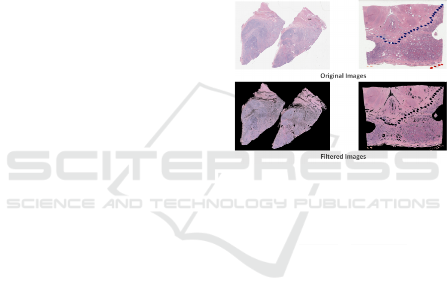
4.2 Data Preprocessing
Since prostate cancer slides with giga-pixel resolution
contain around 50% background regions, we shrink
the slides by a factor of 32 and threshold the fore-
ground pixels (e.g., tissue areas) using OTSU algo-
rithm (Otsu, 2007), which is suitable for tissue area
segmentation. Some prostate cancer slides may have
been contaminated by red, blue or green pen marks.
We filter R, G, B channels respectively with tens of
threshold values to create a mask for tissue area. Mor-
phological operations such as dilation and erosion are
conducted to fill in small blanks and remove outliers.
Then, shrinked images are multiplied with their bi-
nary masks to generate tissue area (Fig. 2). Finally,
a set of patches with size 256*256 are extracted from
tissue area without overlap. Patches that contain less
than 70% tissue regions are discarded from analysis.
4.3 Implementation Details
The implementation details of our experiments are de-
scribed as follows.
(1) Parameter setting for training CNN models as fea-
ture extractor. During training, the batch size is set to
32 and SGD optimizer is used with an initial learn-
ing rate of 1e
−3
. Specifically, all the CNN models are
trained for 20 epochs using a warming up step in the
first 2 epochs, which can further promote the accuracy
of classification.
(2) Parameter setting for GNN based models. We set
3 GCN layers followed by 1 Pooling layer with an
assignment rate of 20%. All the GNN based models
are trained for 1000 epoches using 10-fold validation.
Finally, the batch size and initial learning rate during
training process is set to 20 and 1e
−3
respectively.
4.3.1 Patch Selection
In a histopathology slide, tumor area takes up only
a small ratio of the whole image, automatic Regions
Of Interests (ROIs) selection is crucial for Gleason
grading. In histopathology slides, tumor area means
active mitosis and more nuclei, which appears more
blue while non-tumor area appears more pink or red
(Chang et al., 2011). Blue ratio image (BR image)
corresponds well to this property and was used in pre-
vious research (del Toro et al., 2017) to select relevant
patches. BR value can be calculated as Eq. (9) where
Figure 2: Filtered images. The two images on the top are
original slides shrinked by a factor of 32x. The filtered im-
ages are shown at the bottom.
R, G, B represent the pixel value of red, green, blue
channel respectively.
BR =
100 × B
1 + R + G
×
256
1 + B + R + G
(9)
We rank the patches extracted from one slide ac-
cording to their BR scores, which are calculated by
averaging BR value of every pixel. Usually, tumor
area only accounts for about 10% of the whole tissue
area, thus top 10% patches are regarded as cancerous.
To further reduce the computation cost, 1000 patches
are randomly selected for subsequent processing. For
the slides with less than 1000 cancerous patches, all
of them are accepted. Figure 3 shows an example heat
map created based on BR score, the number of nuclei
in the patch with high BR score is significantly higher
than that in the patch with a lower BR score.
4.3.2 Color Normalization
Color variation is another factor that could damage
the accuracy of GS classification (Abhishek et al.,
2016). Distinct tissue preparation, H & E stain re-
activity, and scanners produced by different man-
ICPRAM 2021 - 10th International Conference on Pattern Recognition Applications and Methods
430

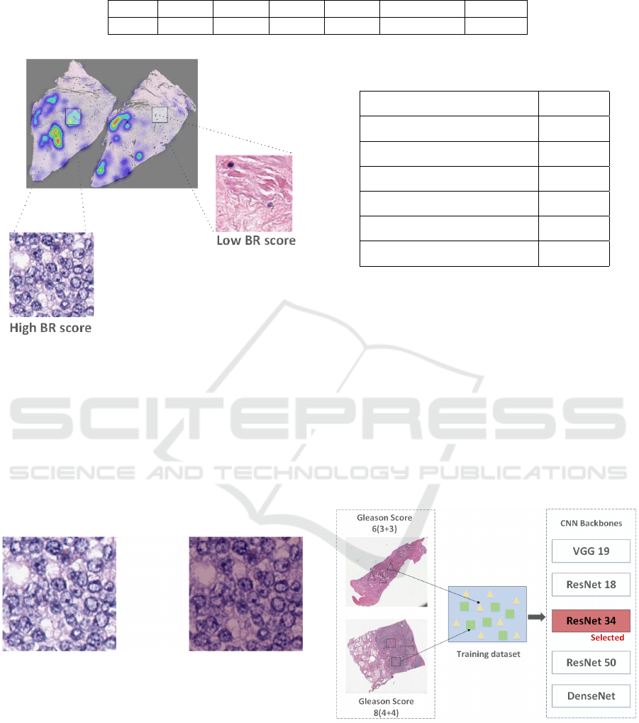
Table 1: The number of prostate cancer slides from TCGA under different GS.
GS 6(3+3) 7(3+4) 7(4+3) 8(4+4) 9 (4+5,5+4) 10(5+5)
#WSI 43 110 84 47 117 5
Figure 3: Patch Selection. The patch with high BR score
appear more blue due to active mitosis while that with low
BR score appear more pink.
ufacturers will result in color variations of digital
histopathology slides. Therefore, color normalization
is performed on selected patches using the color trans-
fer method (Reinhard et al., 2001), which converts
patches into a color template that is determined in
advance, to alleviate the damage of color variations.
Figure 4 shows the comparison of a patch before (left)
and after (right) color normalization.
Figure 4: Color normalization. Image on the left is the orig-
inal patch and the normalized patch is shown on the right.
4.3.3 CNN Feature Extractor
For graph reconstruction, we train a CNN classifier
to extract patch features (Figure 5). To evaluate the
performance of different CNN architectures, VGG19
(Li et al., 2019), ResNet18, ResNet34, ResNet50 (He
et al., 2016) and DenseNet (Huang et al., 2016) are
used as backbones for classification of G3 patches
versus G4 patches. Since our interest lies in classi-
fication of G3 + G4 and G4 + G3, we assume that
Table 2: Classification accuracy of different CNN back-
bones.
Feature Extractor backbones Accuracy
VGG19 77.01%
GoogleNet 77.04%
ResNet18 88.27%
ResNet34 89.42%
ResNet50 85.46%
DenseNet 81.04%
labels of the patches selected from pure slides (e.g.,
G3 + G3 and G4 + G4) are consistent with G3 and
G4.
Table 2 compares the performance of VGG19 (Si-
monyan and Zisserman, 2014), GoogleNet (Szegedy
et al., 2014), ResNets (He et al., 2016) and DenseNet
(Huang et al., 2016). From table 2, we can see that
ResNets have a higher capability to learn useful in-
formation for classification task. As the number of
CNN layer grows, the accuracy first increases and
then starts to decrease. This is because more trainable
parameters yields overfitting. Therefore, the best per-
forming ResNet34 was choosen as our patch feature
extractor.
Figure 5: The training process of feature extractor. We
train the feature extractor using patches extracted from pure
slides (e.g., GS 6(3+3) and GS 8(4+4)).
4.3.4 Graph Reconstruction
We feed patches selected into ResNet34 to get 512
dimensional feature vectors. Then PCA is used to
compress the vectors into 32 dimension to reduce the
Weakly Supervised Gleason Grading of Prostate Cancer Slides using Graph Neural Network
431

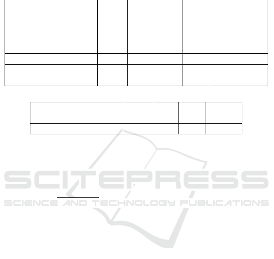
Table 3: Test performance of different models for Gleason grading.
Models Accuracy Dataset F1 score classification task
Nagpal et al. 70.0%
112 million patches
and 1490 slides
-
4 Gleason groups
Zhou et al. 75.0% TCGA - G3 + G4 vs.G4 + G3
GCN + Euclidean 75.3% TCGA 0.720 G3 + G4 vs.G4 + G3
GCN + Euclidean + DIFFPOOL 76.8% TCGA 0.741 G3 + G4 vs.G4 + G3
GCN + Mahalanobis 77.9% TCGA 0.774 G3 + G4 vs.G4 + G3
GCN + Mahalanobis + DIFFPOOL 79.5% TCGA 0.775 G3 + G4 vs.G4 + G3
Table 4: Results of classification of low GS(e.g.,<=GS 7) vs. high GS (e.g., >= GS 8).
Models Accuracy Dataset F1 score #GCN layer
del Toro et al. 78.2% TCGA - -
GCN + Mahalanobis + DIFFPOOL 83.4% TCGA 0.820 3
computation cost. In addition, dense graphs will sig-
nificantly increase the computation cost and sparse
graphs can not accurately model the correlation be-
tween patches. In order to construct graphs with ap-
propriate number of edges, distance threshold is set to
40% of the average distance between all patch pairs in
the edge generation module (e.g., Eq. (10)).
d = 0.4 ×
∑
i, j∈n
Dist(x
i
, x
j
)
C
2
n
(i 6= j)
(10)
Where d is the distance threshold and n denotes the
number of patches that selected from one prostate
cancer slide.
4.4 Results
In this study, we focus on the classification of het-
erogeneous GS 7 and propose a GCN based weakly
supervised Gleason grading model. We construct
edges of graphs using Euclidean and Mahalanobis
distance metrics and train the models with GCN and
GCN+DIFFPOOL as backbones. Our models are
trained for 1000 epochs using 10-fold validation, the
best accuracy and F1-score of each fold are averaged
to obtain the final results. All the results are shown in
table 3 and table 4.
In table 3, we show the performance of different
combinations and results of existing works. We can
see that all GCN based methods give better results
than (Zhou et al., 2017) and (Wang et al., 2018). This
is likely due to the fact that GCN can accurately cap-
ture the relationships among patches and the global
topological information, which are of great signifi-
cance for Gleason grading task. GCN + Mahalanobis
+ DIFFPOOL achieves the best performance with an
accuracy of 79.5%. It approves that DIFFPOOL mod-
ule can help to learn meaningful node clusters by
pooling similar nodes together and obtain the accu-
rate graph representation hierarchically. Table 3 also
reveals that distance metrics make a difference on
the performance of classification of GS 7. Methods
with Mahalanobis metric achieve better results than
those with Euclidean metric, this is because the Ma-
halanobis metric leverages correlations of attributes
of features by introducing the covariance matrix that
shows the correlations of attributes.
To further verify the effectiveness of our devel-
oped method, we apply our model on the classifica-
tion of high GS (e.g., GS ¿= 8) vs. low GS (e.g., GS ¡=
7). The results are shown in table 4. We train the fea-
ture extractor using patches selected from the slides
with GS 6 (G3 + G3), GS 8 (G4 + G4) and GS 10
(G5 + G5). Since we have only 5 slides graded as GS
10, data augmentation including mirroring, random
cropping, rotation, and local warping is conducted.
To save more information about G5, in graph con-
struction process, we use high dimensional node em-
beddings and leave out the PCA process. An accu-
racy of 83.4% is achieved, which is superior to the
result 78.2% of (del Toro et al., 2017). As described
in related work, this is likely due to the fact that they
annotated the patches with slide-level labels directly,
which can seriously damage the accuracy of the clas-
sification of GS 7.
ICPRAM 2021 - 10th International Conference on Pattern Recognition Applications and Methods
432

5 CONCLUSIONS
In this study, we introduce a GCN based model that is
capable of grading the heterogeneous prostate cancer
slides with GS 7 automatically. We construct prostate
cancer slides as graphs to model correlations among
patches and capture topological information of the
whole slides. By combining DIFFPOOL layer with
GCN layers, our method achieves an classification
accuracy of 79.5%, which is superior to state-of-the-
art result on the dataset of TCGA. The reported re-
sults demonstrate efficiency of the proposed method,
which are consistent with our expectation.
ACKNOWLEDGEMENTS
This work was supported in part by the National Key
Research and Development Program of China un-
der Grant 2018YFC0910500, in part by the National
Natural Science Foundation of China under Grant
61906032, in part by the Liaoning Key R&D Program
under Grant 2019JH2/10100030, in part by the Liaon-
ing United Foundation under Grant U1908214, and in
part by the Fundamental Research Funds for the Cen-
tral Universities under Grant DUT20RC(4)005 and
DUT18RC(3)069.
REFERENCES
Abhishek, Vahadane, Tingying, Peng, Amit, Sethi, Shadi,
Albarqouni, Lichao, and and, W. (2016). Structure-
preserving color normalization and sparse stain sepa-
ration for histological images. IEEE transactions on
medical imaging.
Arvaniti, E., Fricker, K. S., Moret, M., Rupp, N. J., Her-
manns, T., Fankhauser, C. D., Wey, N., Wild, P. J.,
Ruschoff, J. H., and Claassen, M. (2018). Automated
gleason grading of prostate cancer tissue microarrays
via deep learning. Scientific Reports, 8(1):12054–
12054.
Bulten, W., Pinckaers, H., Van Boven, H., Vink, R., De Bel,
T., Van Ginneken, B., Jeroen, V. D. L., De Kaa, H. V.,
and Litjens, G. (2019). Automated gleason grading of
prostate biopsies using deep learning.
Chang, H., Loss, L. A., and Parvin, B. (2011). Nuclear seg-
mentation in h & e sections via multi-reference graph
cut ( mrgc ).
del Toro, O. J., Atzori, M., Ot
´
alora, S., Andersson, M.,
Eur
´
en, K., Hedlund, M., R
¨
onnquist, P., and M
¨
uller,
H. (2017). Convolutional neural networks for an au-
tomatic classification of prostate tissue slides with
high-grade Gleason score. In Gurcan, M. N. and
Tomaszewski, J. E., editors, Medical Imaging 2017:
Digital Pathology, volume 10140, pages 165 – 173.
International Society for Optics and Photonics, SPIE.
Epstein and Jonathan, I. (2018). Prostate cancer grading:
a decade after the 2005 modified system. Modern
Pathology An Official Journal of the United States &
Canadian Academy of Pathology Inc, 31:S47.
Epstein, J. I., Egevad, L., Amin, M. B., Delahunt, B.,
Srigley, J. R., and Humphrey, P. A. (2015). The 2014
international society of urological pathology (isup)
consensus conference on gleason grading of prostatic
carcinoma definition of grading patterns and proposal
for a new grading system. The American Journal of
Surgical Pathology, 40(2):244–252.
Epstein, J. I., Zelefsky, M. J., Sjoberg, D. D., Nelson, J. B.,
Egevad, L., Magigalluzzi, C., Vickers, A. J., Parwani,
A. V., Reuter, V. E., Fine, S. W., et al. (2016). A
contemporary prostate cancer grading system: A vali-
dated alternative to the gleason score. European Urol-
ogy, 69(3):428–435.
Gilmer, J., Schoenholz, S. S., Riley, P. F., Vinyals, O., and
Dahl, G. E. (2017). Neural message passing for quan-
tum chemistry.
He, K., Zhang, X., Ren, S., and Sun, J. (2016). Deep resid-
ual learning for image recognition.
Hochreiter, S. and Schmidhuber, J. (1997). Long short-term
memory. Neural Computation, 9(8):1735–1780.
Huang, G., Liu, Z., Laurens, V. D. M., and Weinberger,
K. Q. (2016). Densely connected convolutional net-
works.
Jian, Ren, Kubra, Karagoz, Michael, Gatza, David, J,
Foran, and and, X. (2018). Differentiation among
prostate cancer patients with gleason score of 7 us-
ing histopathology whole-slide image and genomic
data. Proceedings of SPIE–the International Society
for Optical Engineering.
Kallen, H., Molin, J., Heyden, A., Lundstrom, C., and As-
trom, K. (2016). Towards grading gleason score us-
ing generically trained deep convolutional neural net-
works. pages 1163–1167.
Khurd, P., Bahlmann, C., Maday, P., Kamen, A., Gibb-
sstrauss, S. L., Genega, E. M., and Frangioni, J. V.
(2010). Computer-aided gleason grading of prostate
cancer histopathological images using texton forests.
pages 636–639.
Li, J., Li, W., Gertych, A., Knudsen, B. S., Speier, W.,
and Arnold, C. W. (2019). An attention-based multi-
resolution model for prostate whole slide imageclassi-
fication and localization. arXiv: Computer Vision and
Pattern Recognition.
Moch, H., Cubilla, A. L., Humphrey, P. A., Reuter, V. E.,
and Ulbright, T. M. (2016). The 2016 who classifica-
tion of tumours of the urinary system and male genital
organs—part a: Renal, penile, and testicular tumours.
European Urology, 70(1):93–105.
Nagpal, K., Foote, D., Liu, Y., Pohsuan, Chen, Wulczyn, E.,
Tan, F., Olson, N., Smith, J. L., Mohtashamian, A.,
et al. (2018). Development and validation of a deep
learning algorithm for improving gleason scoring of
prostate cancer. arXiv: Computer Vision and Pattern
Recognition.
Otsu, N. (2007). A threshold selection method from gray-
level histograms. IEEE Transactions on Systems Man
& Cybernetics, 9(1):62–66.
Weakly Supervised Gleason Grading of Prostate Cancer Slides using Graph Neural Network
433

Pinckaers, H., Bulten, W., Jeroen, V. D. L., and Litjens, G.
(2020). Detection of prostate cancer in whole-slide
images through end-to-end training with image-level
labels.
Reinhard, Erik, Ashikhmin, Michael, Shirley, Peter, Gooch,
and Bruce (2001). Color transfer between images.
IEEE Computer Graphics & Applications.
Ren, J., Hacihaliloglu, I., Singer, E. A., Foran, D. J., and Qi,
X. (2018). Adversarial domain adaptation for classifi-
cation of prostate histopathology whole-slide images.
11071:201–209.
Siegel, R. L., Miller, K. D., and Jemal, A. (2017). Cancer
statistics, 2017. Ca A Cancer Journal for Clinicians,
67(1).
Simonyan, K. and Zisserman, A. (2014). Very deep con-
volutional networks for large-scale image recognition.
Computer ence.
Szegedy, C., Liu, W., Jia, Y., Sermanet, P., Reed, S.,
Anguelov, D., Erhan, D., Vanhoucke, V., and Rabi-
novich, A. (2014). Going deeper with convolutions.
Wang, J., Chen, R. J., Lu, M. Y., Baras, A. S., and Mah-
mood, F. (2019). Weakly supervised prostate tma clas-
sification via graph convolutional networks. arXiv:
Computer Vision and Pattern Recognition.
Wang, P., Xiao, X., Glissen Brown, J. R., Berzin, T. M.,
Tu, M., Xiong, F., Hu, X., Liu, P., Song, Y., and
Zhang, D. a. (2018). Development and validation of
a deep-learning algorithm for the detection of polyps
during colonoscopy. Nature Biomedical Engineering,
2(10):741–748.
Weinstein, J. N., Collisson, E. A., Mills, G. B., Shaw, K.
R. M., Ozenberger, B., Ellrott, K., Sander, C., Stuart,
J. M., Chang, K., Creighton, C. J., et al. (2013). The
cancer genome atlas pan-cancer analysis project. Na-
ture Genetics, 45(10):1113–1120.
Wu, Z., Pan, S., Chen, F., Long, G., Zhang, C., and Yu,
P. S. (2019). A comprehensive survey on graph neural
networks. IEEE Transactions on Neural Networks and
Learning Systems.
Xu, H., Park, S., and Hwang, T. H. (2018). Automatic
classification of prostate cancer gleason scores from
digitized whole slide tissue biopsies. bioRxiv, page
315648.
Zareba, P., Zhang, J., Yilmaz, A., and Trpkov, K. (2010).
The impact of the 2005 international society of uro-
logical pathology (isup) consensus on gleason grading
in contemporary practice. Histopathology, 55(4):384–
391.
Zhang, Y. H., Zhang, J., Song, Y., Shen, C., and Yang, G.
(2020). Gleason score prediction using deep learning
in tissue microarray image. arXiv e-prints.
Zhou, N., Fedorov, A., Fennessy, F. M., Kikinis, R., and
Gao, Y. (2017). Large scale digital prostate pathology
image analysis combining feature extraction and deep
neural network. arXiv: Computer Vision and Pattern
Recognition.
ICPRAM 2021 - 10th International Conference on Pattern Recognition Applications and Methods
434