Mathematical Model for Estimating Nutritional Status of the Population

with Poor Data Quality in Developing Countries: The Case of Chile

Denisse

Avalos

, Crist

obal Cuadrado

2,3 a

, Jocelyn Dunstan

4,5 b

, Javier Moraga-Correa

1,6

Luis Rojo-Gonz

alez

1,7 c

, Nelson Troncoso

and

Oscar C. V

asquez

1 d

Department of Industrial Engineering, Universidad de Santiago, Santiago, Chile

School of Public Health, Universidad de Chile, Santiago, Chile

Centre for Health Economics, University of York, York, U.K.

Center for Mathematical Modeling - CNRS UMI2807, Universidad de Chile, Santiago, Chile

Center for Medical Informatics and Telemedicine, Universidad de Chile, Santiago, Chile

Business School, University of Nottingham, Nottingham, U.K.

Facultat de Matem

atiques i Estad

ıstica, Universitat Polit

ecnica de Catalunya, Barcelona, Spain

Keywords:

Transition Probabilities, Obesity, Developing Countries, Non-linear Programming, Poor Data Quality.

Abstract:

Obesity is one of the most important risk factors for non-communicable diseases. Nutritional status is gen-

erally measured by the body mass index (BMI) and its estimation is especially relevant to analyse long-term

trends of overweight and obesity at the population level. Nevertheless, in most context nationally represen-

tative data on BMI is scarce and the probability of individuals to progress to obese status is not observed

longitudinally. In the literature, several authors have addressed the problem to obtain this estimation us-

ing mathematical/computational models under a scenario where the parameters and transition probabilities

between nutritional states are possible to compute from regular ofﬁcial data. In contrast, the developing coun-

tries exhibit poor data quality and then, the approaches provided from the literature could not be extended to

them. In this paper, we deal with the problem of estimating nutritional status transition probabilities in settings

with scarce data such as most developing countries, formulating a non-linear programming (NLP) model for

a disaggregated characterization of population assuming the transition probabilities depend on sex and age.

In particular, we study the case of Chile, one of the countries with the highest prevalence of malnutrition in

Latin America, using three available National Health Surveys between the years 2003 and 2017. The obtained

results show a total absolute error equal to 5.11% and 10.27% for sex male and female, respectively. Finally,

other model applications and extensions are discussed and future works are proposed.

1 INTRODUCTION

The nutritional status of the population is generally

measured using the body mass index (BMI). This

metric is deﬁned as the weight divided by height

squared, kg/m

(Okorodudu et al., 2010; Apovian,

2016). In contrast to other technical metrics such

as dual-energy x-ray absorptiometry, BMI is easy-

to-implement in clinical practice and population sur-

veys and provides a similar discriminatory capability

https://orcid.org/0000-0002-0174-5958

https://orcid.org/0000-0001-6726-7242

https://orcid.org/0000-0003-4894-2470

https://orcid.org/0000-0002-1393-4692

(Huxley et al., 2010; NCD Risk Factor Collaboration

(NCD-RisC), 2016; NCD Risk Factor Collaboration

(NCD-RisC), 2017). In practice, this metric allows to

classify the nutritional status for individuals aged 18

years and older according to its BMI into four groups

proposed by the World Heath Organization (WHO): i)

Underweight, BMI < 18.4; ii) Normal, 18.5 ≤ BMI

≤ 24.9; iii) Overweight, 25.0 ≤ BMI ≤ 29.9; and iv)

Obese, BMI ≥ 30.

Unfortunately, obesity represents one of the most

important risk factors for non-communicable dis-

eases. It was declared an epidemic in 1990 by the

World Health Organization, reaching the ﬁrst position

in the 21st century. Between the years 1995 and 2000,

408

Ávalos, D., Cuadrado, C., Dunstan, J., Moraga-Correa, J., Rojo-González, L., Troncoso, N. and Vásquez, Ó.

Mathematical Model for Estimating Nutritional Status of the Population with Poor Data Quality in Developing Countries: The Case of Chile.

DOI: 10.5220/0010262404080415

In Proceedings of the 10th International Conference on Operations Research and Enterprise Systems (ICORES 2021), pages 408-415

ISBN: 978-989-758-485-5

adult population with obesity increased in 100 mil-

lion people, reaching 300 million worldwide, whereas

18 million under-ﬁve year children have overweight

(World Health Organization, 2003). In addition, more

than 1.9 billion adults aged 18 years and older were

overweight, being 650 million adults were obese in

2016 (World Health Organization, 2016).

Consequently, the estimation of the prevalence of

different nutritional status categories is especially rel-

evant for the development of future health policies

due to at least two reasons:

• Obesity is associated with the leading causes of

death worldwide since the management of its re-

lated factors has proven to be tremendously com-

plex presenting a sustained upward trend. In par-

ticular, obesity is related to serious health risks

(National Institutes of Health, 1998). For in-

stance, every 5-unit increases in BMI above 25,

the overall mortality increases by 29%, cardiovas-

cular mortality by 41%, and diabetes-related mor-

tality by 210% (Apovian, 2016).

• In terms of the associated costs, a person who

has obesity incurs an annual healthcare cost of

36% greater than a normal weight person and a

77% higher in the medication costs (Sturm, 2002).

In this sense, some authors have been reported

that an obese patient has annual medical spending

between 25% (Detournay et al., 2000) and 42%

(Finkelstein et al., 2003) higher than who is of

normal weight. This account for direct costs of,

at least, 5%, of the total health expenditures of

developed countries (Levy et al., 1995; Manson

et al., 2004). In practice, if the number of indi-

viduals aged 16 and 17 who have overweight or

obesity could be reduced by 1%, this would re-

sult in a decrease in lifetime medical costs of $586

million (Wang et al., 2010). In addition, it might

be expected that at low-income levels of the coun-

try the underweight prevalence should dominate

the landscape, but the projected average annual

growth of obesity indicates that, across 147 coun-

tries, it will increase 2.47% respect to the Gross

Domestic Product per capita during 2019-2024

(Talukdar et al., 2020).

The problem of estimation of long-term trends of obe-

sity prevalence is mainly addressed by using mathe-

matical models that aim to capture the relationships

among environment, biological, social and cultural

aspect from a system point of view under a scenario

where regular ofﬁcial data is available (Mitchell et al.,

2011; Frerichs et al., 2013). However, these ap-

proaches could not be easily extended to other settings

where the data is not collected regularly or not exten-

sively enough. For instance, the developing countries

such as Argentina (Secretar

ıa de Gobierno de Salud,

Argentina, 2019), Brazil (Instituto Brasileiro de Ge-

ograf

ıa e Estad

ıstica, Brasil, 2020), Colombia (Min-

isterio de Salud, Colombia, 2015) and Chile (Ministe-

rio de Salud, Chile, 2017) only provide two and three

national health survey into two decades.

1.1 Literature Review

In the literature, the importance of estimating obesity

prevalence over time and how to use National Health

Surveys in each country as main data source, is em-

phasized from different modeling perspectives (see

(Olariu et al., 2017) for a recent survey in Markov

cohort models and (Xue et al., 2018) for a recent sur-

vey in system dynamic (SDM) and agent-based mod-

eling (ABM)). In particular, the researchers mention a

special key input called transition probabilities in the

chronic disease modeling context. They are deﬁned as

the probability or rate to move from one state of a cat-

egorical risk factor (e.g. nutritional status) to another

(Van de Kassteele et al., 2012); being transition rates

and transference rates sometimes used as synonyms.

In the last decades, several authors have addressed

the estimation of the nutritional status for the pop-

ulation from developed countries. For instance, a

multi-stage Markov model is decribed in (Van de

Kassteele et al., 2012), which is used on the “Perma-

nent Onderzoek Leef Situatie” data for the Nether-

lands collected between 2006 and 2007, that is to

say, a cross-sectional study, considering the individ-

uals of 85 years old tops. To compute the transi-

tion probabilities the authors consider a transportation

problem (well-known in Linear Programming), where

the results show that the prevalence of being normal

weight during the last year and have obesity the next

year, and vice versa, is null at any age. A suscep-

tible–infected–recovered model for the United States

(US) and the United Kingdom (UK) is proposed in

(Ward et al., 2017), using the information between

1988 and 1998 (Ogden et al., 2006), and the Health

Survey for England between 1993 and 1997 (Thomas

et al., 2014), respectively; indicating that, via a for-

ward simulation, the obesity prevalence will plateau

independent of current prevention strategies at 32%

(US) and 39.6% (UK) by about 2030. A longitudinal

study, from an ABM simulation point of view, was

carried out using the National Health and Nutrition

Examination Survey from 1976 through 2014 to pre-

dict risk factors for the nutritional statuses for indi-

viduals aged 35 years. The results project that a ma-

jority of children (57.3%) will be obese at the age of

35 years, and roughly half of the projected prevalence

will occur during childhood.

Mathematical Model for Estimating Nutritional Status of the Population with Poor Data Quality in Developing Countries: The Case of Chile

409

Recently, several authors have tackled the prob-

lem of estimating the nutritional status of the popu-

lation with poor data quality. A time-homogeneous

continuous-time Markov model is proposed in (Lartey

et al., 2020) to compute the transition probabilities

between nutritional statuses, using the Ghana Who

SAGE in 2007/2008 and 2014/2015. The obtained re-

sults show that, for obese individuals, the probability

of remaining obese, decrease to overweight and nor-

mal weight was 90.2%, 9.2%, and 0.6%, respectively.

Complementary to the previous works in this ﬁeld,

our research acknowledges the reality of the so-called

developing countries, where the data is not collected

regularly or not very extensively.

1.2 Our Contribution

This research deals with the problem of estimating

the nutritional status of the population with poor data

quality in developing countries. In particular, we

study the case of Chile, which ranks third in Latin

America in child overweight prevalence with a pres-

ence of 9.3% (Food and Agriculture Organization,

2018) and second among the countries of the Orga-

nization for Economic Cooperation and Development

in overweight prevalence for the population over 15

years old. Chile represents an example where the data

is not collected regularly or not very extensively, as it

is often the case in other regions of the ’developing’

world. Formally, we formulate a non-linear program-

ming (NLP) model, which allows us to determine the

transition probabilities considering a set of disaggre-

gated variables by BMI and age ranges and assum-

ing the transition probabilities depend on sex and age

range. The parameters are obtained from the analysis

of the ofﬁcial reports and the three available national

health surveys between the years 2003 and 2017. To

test the performance of our NLP model, we carry out

computational experiments and compute the total ab-

solute error of our estimation in different scenarios.

Finally, other applications for the model are discussed

and future works are proposed.

2 NON-LINEAR PROGRAMMING

(NLP) MODEL

2.1 Dynamic Conceptualization

In order to deﬁne our model, we introduce the dy-

namic conceptualization for the population’s nutri-

tional status during a given period. Let I , J and K

be the sets of discretized BMI, age ranges, and sexes,

respectively. For convenience, we denote T the set of

the years within the given period and the state of the

population is deﬁned by BMI i, age range j, and sex k.

From each state, the movements within and between

the BMI and age ranges are modeled according to the

transition probabilities. We distinguish the transition

probabilities to decrease, to remain or to increase the

current BMI as follow: i) α

j,k

, is the transition proba-

bility to increase the BMI of the people of sex k from

the year t to the year (t + 1); ii) β

j,k

, is the transition

probability to decrease the BMI of the population of

sex k from one year t to the year (t + 1) and iii) φ

j,k

is the transition probability to remain the BMI of the

population of sex k from one year t to the year (t +1).

In addition, we consider the population growth

i, j,k

and the population proportion γ

j,k

of sex k in the

upper bound of the age range j at year t (i.e., the pop-

ulation proportion that would change their age range

from year t to year (t + 1)). Note that this proportion

is assumed equal to 0% in the last age range. Thus, the

transition probabilities for the above population pro-

portion can be separated into two sub-categories as

follow: i) η

α,t

j,k

:= γ

j,k

, η

β,t

j,k

:= γ

j,k

and η

φ,t

j,k

as the transition probabilities to increase, to

decrease or to remain the BMI from year t to the year

(t +1) but, at the same time, changing their age range;

and ii) ψ

α,t

j,k

:= (1−γ

j,k

)α

j,k

, ψ

β,t

j,k

:= (1−γ

j,k

)β

j,k

and

φ,t

j,k

:= (1 − γ

j,k

)φ

j,k

as the transition probabilities to

increase, to decrease or to remain the BMI from year

t to the next one (t +1) but, at the same time, remain-

ing their age range. An illustration of the dynamic

conceptualization is shown in Figure 1.

Figure 1: Illustration of the dynamic conceptualization.

Two consecutive years, t and t + 1 are depicted in order to

show the transitions of some deﬁned population.

ICORES 2021 - 10th International Conference on Operations Research and Enterprise Systems

410

2.2 Formulation

We denote I

i, j,k

the continuous positive variable that

represents the population of BMI i ∈ I , age range j ∈

J and sex k ∈ K at year t ∈ T . Let T and T be the

bounds on the years in the model. The model aims

to minimize the weighted mean squared error in the

ﬁtting of the population during the period in [T ;T ].

We deﬁne w

j,k

as the population proportion of sex k ∈

K in age range j ∈ J at the end of the year T . Let

i, j,k

be the real population at the end year T . Given

a sex k ∈ K , the NLP model is deﬁned as follows:

[MIN]

∑

i∈I

∑

j∈J

i, j,k

−U

i, j,k

)

j,k

(1)

subject to (for each year t ∈ {T ...T − 1})

t+1

i, j,k

1 − κ

i, j,k

=ψ

α,t

j,k

i−1, j,k

+ +η

α,t

j−1,k

i−1, j−1,k

+ ψ

φ,t

j,k

i, j,k

+ η

φ,t

j−1,k

i, j−1,k

+ ψ

β,t

j,k

i+1, j,k

+ η

β,t

j−1,k

i+1, j−1,k

∀ j ∈ J \ {1}, ∀i ∈ I \ {1,|I |} (2)

j,k

=η

α,t

j,k

+ η

β,t

j,k

+ η

φ,t

j,k

∀ j ∈ J (3)

(1 − γ

j,k

) =ψ

α,t

j,k

+ ψ

β,t

j,k

+ ψ

φ,t

j,k

∀ j ∈ J (4)

min

j,k

≤ η

α,t

j,k

+ ψ

α,t

j,k

≤ α

max

j,k

∀ j ∈ J (5)

min

j,k

≤ η

β,t

j,k

+ ψ

β,t

j,k

≤ β

max

j,k

∀ j ∈ J (6)

min

j,k

≤ η

ψ,t

j,k

+ ψ

ψ,t

j,k

≤ φ

max

j,k

∀ j ∈ J (7)

i, j,k

,η

α,t

j,k

,η

β,t

j,k

,η

φ,t

j,k

,ψ

α,t

j,k

,ψ

β,t

j,k

,ψ

φ,t

j,k

≥ 0 ∀i ∈ I , j ∈ J (8)

Expression (1) states the objective function of the

model. The possible transition is deﬁned by the set

of constraints (2). These transitions are constrained

to the proportion to change of age range given by the

set of constraints (3)–(4), the bounds on these tran-

sitions are imposed by the set of constraints (5)–(7)

and the domain of the variables is deﬁned in the set of

constraints (8).

2.3 Discretization and Data Wrangling

To compute the required parameters, we consider

ofﬁcial reports such as the three collected National

Health Surveys (ENS) into 15 years provided by the

Ministry of Health of Chile (MINSAL) (Ministerio

de Salud, Chile, 2017), the governmental documents

from the Department of Statistics and Health Infor-

mation (DEIS) (Departamento de Estad

ıstica e Infor-

maci

on de Salud, 2018) and the National Institute

of Statistics (INE) (Instituto Nacional de Estad

ıstica,

2017). Since the proposal required a discretization of

the variables, we should do it to achieve the desired

shape of the input. Thus, we consider the BMI as the

integer value of the recorded value and to group the

age by ranges of 10 years starting from 15 years old

such as a population grid is obtained.

However, as the survey is only a sample of the

entire population, there would likely be some com-

binations of the grid that have zero-counting. There-

fore, we should avoid this ﬁrst issue by redistribut-

ing the population. So, the discussion now turns into

which model to pick and how to set its parameters.

Even although we should deal with a bi-variate distri-

bution over the BMI and the age range, there is not

evidence of this, but it does by considering the BMI

itself. For instance, it is common to assume a Gaus-

sian distribution, but it would be true if and only if

the related multi-factorial processes have additive ef-

fects; nonetheless, for biologic variables, the knowl-

edge suggests that these processes have a multiplica-

tive effect, e.g., an obesogenic environment, which is

more likely to follow a skewed, possibly log-normal,

distribution (Penman and Johnson, 2006).

A particular analysis is carried out on the popula-

tion growth, κ

i, j,k

. The population growth is the dif-

ference between the birth rate and the mortality rate

and, as we are considering people older than 15 years

old, it is necessary to get this rate in a time-lagged

sense, i.e., we need the birth rate of the people that

were born 15 years ago. Besides, a requirement is that

this rate should be distributed by BMI and age ranges.

Addressing this latter issue, from a separable point of

view, we have that: i) the lagged birth rate only in-

ﬂuences on the ﬁrst age range whereas the mortality

rate is in the whole set of age ranges; ii) to get the

distributed population growth, we use a study related

to survival analysis which works on the Hazard ratios

(Berrington de Gonz

alez et al., 2010) to get them by

BMI.

Even although the transition probabilities are the

core of the study itself, we must provide the feasible

bounds for the estimation. Several authors have been

reported evidence on the transition probabilities for a

speciﬁc nutritional status (Power et al., 1997; Orpana

et al., 2006; Laitinen et al., 2001; Booth et al., 2012;

Fildes et al., 2015; Srinivasan et al., 1996). However,

the obtained results reported by them are not neces-

sarily the BMI and age range considered. To address

this problem, we propose to work with multiple sce-

narios approach from the literature data. Thus, the

bounds of the transition probabilities, X, and its mean

value, Ave(X ), are assumed to be normal distributed

such that the conﬁdence bounds of the transition prob-

ability, say Ave(X ) as the lower bound, and Ave(X) as

the upper bound, at a conﬁdence level δ% can be ob-

tained from Pr(Ave(X) ≤ X ≤ Ave(X)) = δ.

Mathematical Model for Estimating Nutritional Status of the Population with Poor Data Quality in Developing Countries: The Case of Chile

411

3 RESULTS

The computational experiments are carried out split-

ting up the data into a ﬁtting period (2003-2010) and

a validation period (2010-2017) as a forward simula-

tion to set out the performance of the model.

3.1 Implementation

The mathematical model is implemented in AMPL

programming language with Minos as the solver and

executed on a MacBook Air Intel i5, 1.6 GHz, 8GB

RAM, with no stopping time, 2500 iterations tops

considering ﬁve random seeds given the non-linearity

of the model. The obtained results are such that we

use to make a discrete grid at conﬁdence levels in

[0.01;0.995] such as 256 and 254 scenarios are given

with solving time of 38.96 minutes and 41.90 minutes

for males and females, respectively.

3.2 Transition Probabilities

The obtained results show that there are some differ-

ences between the sexes. In particular, such as Table 1

shows, we can see that the standard deviation for each

ﬁtted parameter is quite similar between sexes and the

comparison between them shows a remarkable differ-

ence over the age ranges but not at all. For instance,

while the transition probability to remain the current

BMI is the highest one, the transition probability to

increase the BMI is greater than to decrease until the

65 years old for both sexes but between 65 and 74

years old, the sex female reverses this trend, i.e., the

transition probability to increase the BMI is greater

than to decrease, then this relation gets reverse and

then goes back to the same.

A second important remark concerns the density

of the results (see Figure 2). In fact, the transition

probabilities are ever in the same order; in decreasing

order, they are to remain, to increase, and to decrease.

So, in general, although the transition probability to

remain the current BMI dominates the others, this ef-

fect does not make the difference due to remain a sta-

tus is possible at any level and if we compare from one

year to another it means that the population has a sta-

ble BMI, but when we make the period wider, e.g., 2

years, if the person increases its BMI in the ﬁrst place

and then remains it, the overall effect is that the per-

son increases its BMI from the beginning of the study.

Therefore, it is clear that the population, in the long-

term sense, has a trend to increase their BMI, but im-

portant differences especially exist for sex male and

some age ranges, including ones where the transition

probabilities to decrease or to increase are almost the

same.

For both sexes there is an age range that changes

with respect to the others, for sex male, it is 55-64

years old and for sex female, it is 15-24 years old.

These age ranges have completely different shapes of

the distribution; in fact, they are, from a biological

point of view, interesting phases of hormonal changes

in the body, so they should be carefully analyzed. On

the other hand, for both sexes, a useful remark is re-

lated to the variability and the shape of the transition

probabilities. The distributions are wide enough to

cover the half of the probabilities, at least, whereas

there are not bi-modal ones except the distributions

for the ﬁrst age range. However, the entire previous

comments are just true if the ﬁtting is well. Using

the total absolute error as a metric to compare the

forecasting population against the real population in

2017, it reaches a 5.11% and 10.27% for sex male and

female, respectively. Even when the numbers seem

quite well, it is necessary to see the behavior of the

estimation. Figure 3 depicts, by sex, the real popu-

lation at each BMI (points) and the ﬁtted curve ob-

tained from the model (lines) including their respec-

tively 95% conﬁdence intervals at the end of the ﬁt-

ting period (2010) and at the end of the validation

period (2017). The comparison shows quite similar

behavior and, with low total absolute error for both

sexes, and the fact that the real data belongs to the

conﬁdence intervals (which are not too wide), the ﬁt-

ting might be understood as a good one but taking into

account that both periods differ from each other.

4 DISCUSSION AND FUTURE

WORK

This work addressed the problem of estimating nutri-

tional status with poor data quality. A non-linear pro-

gramming model is formulated to obtain the transition

probabilities that are key elements in the modeling of

this epidemic and the designing of malnutrition public

policy options and the computation of the associated

costs of a speciﬁc population. Our proposal provides

a novel methodology to estimate them with a few data

available and a disaggregated characterization of the

population by sex, BMI and age ranges, in contrast to

other similar work works.

In particular, the research was focused on the

case of Chile, one of the countries with the highest

malnutrition in Latin America. The obtained results

show the ﬁtted transition probabilities are fair via a

straight comparison against the last known informa-

tion. Nonetheless, it is important to say that, despite

ICORES 2021 - 10th International Conference on Operations Research and Enterprise Systems

412

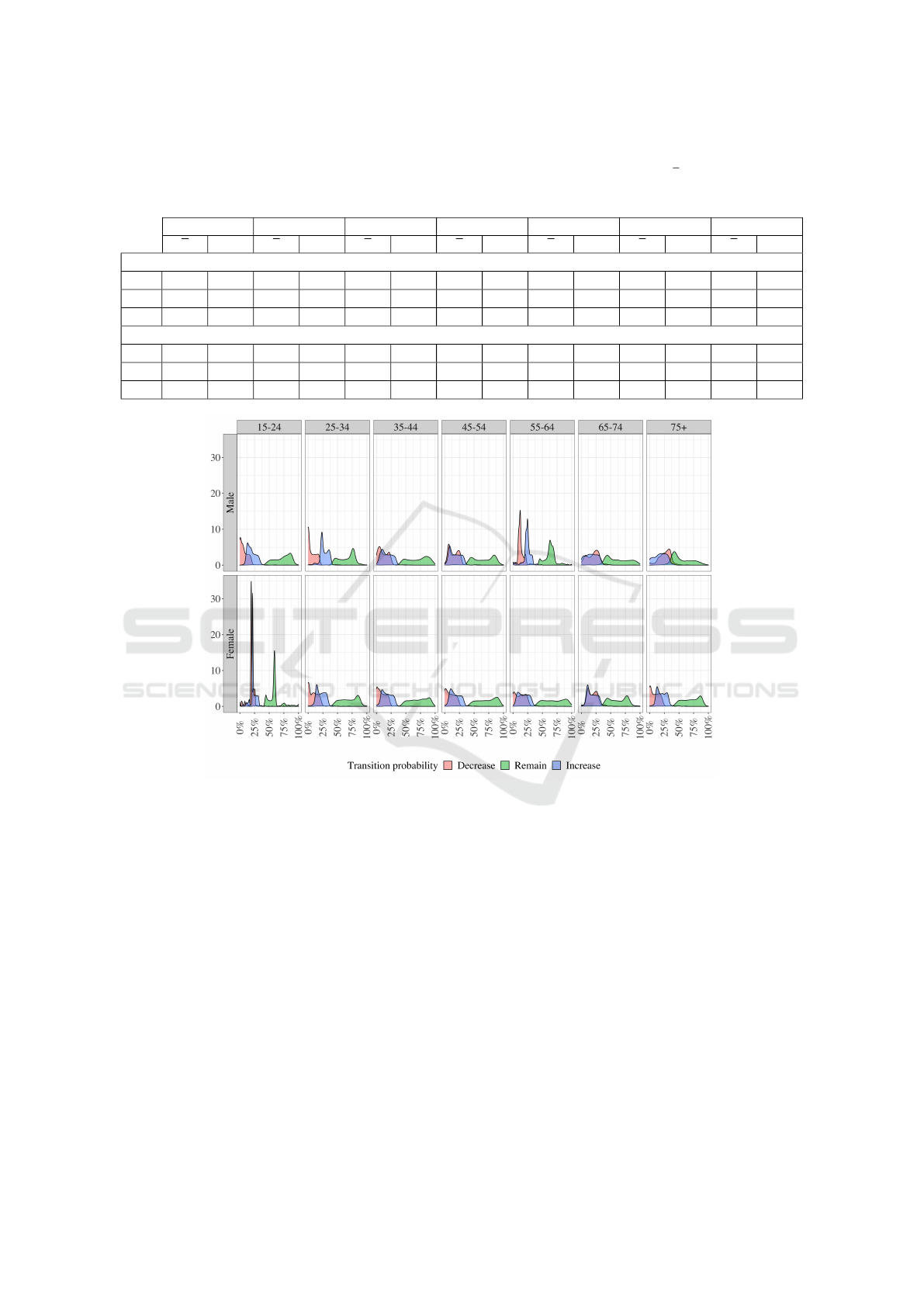
Table 1: Summary of the transition probabilities by sex and age ranges considering the whole ﬁtting period (2003-2010). The

standard deviation (Sd) for each ﬁtted value is similar between sexes. The comparison, in mean (x) terms, shows that the

transition probability to increase the BMI is greater than to decrease until the 65 years old for both sexes but between 65 and

74 years old, the female sex reverses this trend.

15-24 25-34 35-44 45-54 55-64 65-74 75+

x Sd x Sd x Sd x Sd x Sd x Sd x Sd

Male

j,.

7.5 7.6 6.7 7.3 11.9 9.3 15.8 9.4 13.8 8.0 19.8 10.6 26.4 10.3

j,.

71.5 15.7 65.2 15.2 69.7 18.4 65.3 18.6 62.1 12.4 62.1 19.5 54.8 17.2

j,.

20.6 8.3 27.8 8.0 17.8 9.9 18.0 9.9 24.5 8.2 17.7 11.0 18.6 10.4

Female

j,.

19.9 8.4 9.1 8.6 9.8 8.7 11.0 10.7 13.3 11.4 20.4 11.3 10.2 9.6

j,.

57.7 14.1 67.9 16.9 70.5 17.1 69.8 18.8 67.8 19.9 60.8 17.9 68.9 16.9

j,.

23.4 8.5 22.4 9.3 18.6 9.3 18.7 10.2 18.8 10.5 19.1 9.4 21.0 8.7

Figure 2: Distribution of the transition probabilities obtained for the ﬁtting period (2003-2010) by age range and sex. The

transition probabilities are ever in the same order; in decreasing order, they are Remain, Increase, Decrease; but via look-up

analysis, we can suspect that this particular population tends to increase their BMI due to remaining a status just implies

non-changes when the study is at short-term.

the low error in the ﬁtting period, the variability of

the transition probabilities distribution can make them

noisy and their interpretation might be carefully done.

However, the level of disaggregation of the variables

plays an important role in it. Thus, on the assumption

that the transition probabilities are constant within a

particular period and that they do depend on the age

and sex of the person, we get that the population un-

der study has a clear trend, in the long-term sense,

to increase their BMI, but it seems to be some vari-

ables that are not included yet. Besides, note that

the non-linearity of the mathematical model plays an

important role since the non-integer variables cannot

be solved. Also, the lack of information, especially

the time windows for collecting the data, is an im-

portant problem that adds noise to the model when

non-stationary variables are considered. Also, an im-

portant discussion must be done about the obtained

results, where it is known that any long-term forecast-

ing or extrapolation may be wrong when the period

gets longer. In this case, we can see an excellent esti-

mation at ﬁrst glance in the ﬁtting period, but the fore-

casting suffers a change of trend, especially for sex

female, in the validation period. Anyway, the tran-

sition probabilities distribution shows that there are

differences not just between sexes, but between age

ranges as well. In general terms, two age ranges that

have a remarkable change of shape, at 55-64 years

Mathematical Model for Estimating Nutritional Status of the Population with Poor Data Quality in Developing Countries: The Case of Chile

413

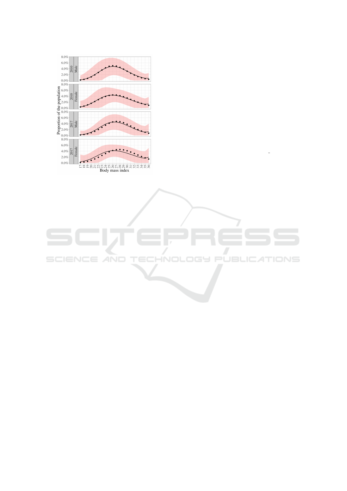
Figure 3: Comparison of the population obtained at the end

of the ﬁtting period (2010) with a 5.11% of total absolute

error, and that one obtained from the forward simulation at

the end of the validation period (2017) with a 10.27% total

absolute error, by sex. The ﬁgure shows the known data

as points and the ﬁtted values are shown as lines, whereas

the shaded area around them represents the 95% conﬁdence

interval.

old for sex men and at 15-24 years old for sex female.

Those age ranges might be associated with hormonal

changes in the body for the respective sex, such as

the andropause for sex male (Tan and Pu, 2002) and

the menstrual cycle for sex female (Van Hooff et al.,

2004). Finally, we propose to explore the transition

probabilities estimation by relaxing the assumption

on the constant behavior according to the current BMI

and to consider non-constant variables based on a dif-

ferent point of view as the Bayesian analysis.

ACKNOWLEDGEMENTS

The authors are grateful for partial support from

the following sources: ANID Beca Mag

ıster en

el Extranjero, Becas Chile, Folio 73190041 (Javier

Moraga-Correa) and Folio 73201112 (Luis Rojo-

Gonz

alez), CONICYT-FONIS SA14ID0176 and

RCUK-CONICYT Newton-Picarte MR /N026640/1

(Crist

obal Cuadrado), CMM-ANID AFB 170001 and

CIMT-CORFO Cost Center 570111 (Jocelyn Dun-

stan), Universidad de Santiago de Chile, Proyecto DI-

CYT 061817VP (

Oscar C. V

asquez).

REFERENCES

Apovian, C. (2016). Obesity: deﬁnition, comorbidities,

causes, and burden. The American Journal of Man-

aged Care, 22(7 Suppl):s176–85.

Berrington de Gonz

alez, A., Hartge, P., Cerhan, J., et al.

(2010). Body-mass index and mortality among 1.46

million white adults. The New England Journal of

Medicine, 363(23):2211–2219.

Booth, H., Prevost, A., and Gulliford, M. (2012). Epi-

demiology of clinical body mass index recording in

an obese population in primary care: a cohort study.

Journal of Public Health, 35(1):67–74.

Departamento de Estad

ıstica e Informaci

on de Salud

(2018). Defunciones. https://public.tableau.com/

proﬁle/deis4231#!/vizhome/Anuario Defunciones/

Defunciones. Online; accessed 3 oct 2020.

Detournay, B., Fagnani, F., Phillippo, M., et al. (2000).

Obesity morbidity and health care costs in France: an

analysis of the 1991-1992 medical care household sur-

vey. International Journal of Obesity, 24(2):151–155.

Fildes, A., Charlton, J., Rudisill, C., et al. (2015). Probabil-

ity of an obese person attaining normal body weight:

cohort study using electronic health records. Ameri-

can Journal of Public Health, 105(9):e54–e59.

Finkelstein, E., Fiebelkorn, I., and Wang, G. (2003). Na-

tional medical spending attributable to overweight and

obesity: How much, and who’s paying? further evi-

dence that overweight and obesity are contributing to

the nation’s health care bill at a growing rate. Health

Affairs, 22(Suppl1):219–226.

Food and Agriculture Organization (2018). Panorama de la

seguridad alimentaria y nutricional en am

erica latina

y el caribe.

Frerichs, L., Araz, O., and Huang, T. (2013). Modeling

social transmission dynamics of unhealthy behaviors

for evaluating prevention and treatment interventions

on childhood obesity. PloS One, 8(12):e82887.

Huxley, R., Mendis, S., Zheleznyakov, E., et al. (2010).

Body mass index, waist circumference and waist: hip

ratio as predictors of cardiovascular risk—a review of

the literature. European Journal of Clinical Nutrition,

64(1):16–22.

Instituto Brasileiro de Geograf

ıa e Estad

ıstica, Brasil

(2020). Pesquisa Nacional de Sa

ude - PNS.

https://www.ibge.gov.br/estatisticas/sociais/

justica-e-seguranca/9160-pesquisa-nacional-de-

saude.html?edicao=9177&t=o-que-e. Online;

accessed 3 oct 2020.

Instituto Nacional de Estad

ıstica (2017). Proyecciones de

Poblaci

on. https://www.ine.cl/estadisticas/sociales/

demograﬁa-y-vitales/proyecciones-de-poblacion.

Online; accessed 3 oct 2020.

Laitinen, J., Power, C., and J

arvelin, M. (2001). Family so-

cial class, maternal body mass index, childhood body

mass index, and age at menarche as predictors of adult

obesity. The American Journal of Clinical Nutrition,

74(3):287–294.

Lartey, S., Lei, S., Otahal, P., et al. (2020). Annual tran-

sition probabilities of overweight and obesity in older

ICORES 2021 - 10th International Conference on Operations Research and Enterprise Systems

414

adults: Evidence from world health organization study

on global ageing and adult health. Social Science &

Medicine, 247:112821.

Levy, E., L

evy, P., Le, C., et al. (1995). The economic cost

of obesity: the French situation. International Journal

of Obesity and Related Metabolic Disorders: Journal

of the International Association for the Study of Obe-

sity, 19(11):788–792.

Manson, J., Skerrett, P., Greenland, P., et al. (2004). The es-

calating pandemics of obesity and sedentary lifestyle:

a call to action for clinicians. Archives of Internal

Medicine, 164(3):249–258.

Ministerio de Salud, Chile (2017). Base de datos. http://

epi.minsal.cl/bases-de-datos/. Online; accessed 3 oct

2020.

Ministerio de Salud, Colombia (2015). Gesti

del conocimiento y fuentes de informaci

on.

https://www.minsalud.gov.co/salud/publica/

epidemiologia/Paginas/gestion-del-conocimiento-y-

fuentes-de-informacion.aspx. Online; accessed 3 oct

2020.

Mitchell, N., Catenacci, V., Wyatt, H., et al. (2011). Obe-

sity: overview of an epidemic. Psychiatric Clinics,

34(4):717–732.

National Institutes of Health (1998). Clinical guidelines for

the identiﬁcation, evaluation, and treatment of over-

weight and obesity in adults - the evidence report.

Obesity Reviews, 6(2):51S–209S.

NCD Risk Factor Collaboration (NCD-RisC) (2016).

Trends in adult body-mass index in 200 countries from

1975 to 2014: a pooled analysis of 1698 population-

based measurement studies with 19.2 million partici-

pants. The Lancet, 387(10026):1377–1396.

NCD Risk Factor Collaboration (NCD-RisC) (2017).

Worldwide trends in body-mass index, underweight,

overweight, and obesity from 1975 to 2016: a pooled

analysis of 2416 population-based measurement stud-

ies in 128.9 million children, adolescents, and adults.

The Lancet, 390(10113):2627–2642.

Ogden, C., Carroll, M., Curtin, L., et al. (2006). Prevalence

of overweight and obesity in the United States, 1999-

2004. JAMA, 295(13):1549–55.

Okorodudu, D., Jumean, M., Montori, V., et al. (2010). Di-

agnostic performance of body mass index to identify

obesity as deﬁned by body adiposity: a systematic re-

view and meta-analysis. International Journal of Obe-

sity, 34(5):791–799.

Olariu, E., Cadwell, K., Hancock, E., et al. (2017). Current

recommendations on the estimation of transition prob-

abilities in markov cohort models for use in health

care decision-making: a targeted literature review.

ClinicoEconomics and Outcomes Research: CEOR,

9:537–546.

Orpana, H., Tremblay, M., and Fin

es, P. (2006). Trends

in Weight Change Among Canadian Adults: Evidence

from 1996/1997 to 2004/2005 National Population

Health Survey. Citeseer.

Penman, A. and Johnson, W. (2006). The changing shape

of the body mass index distribution curve in the popu-

lation: implications for public health policy to reduce

the prevalence of adult obesity. Preventing Chronic

Disease, 3(3).

Power, C., Lake, J., and Cole, T. (1997). Body mass index

and height from childhood to adulthood in the 1958

british born cohort. The American Journal of Clinical

Nutrition, 66(5):1094–1101.

Secretar

ıa de Gobierno de Salud, Argentina

(2019). 2° Encuesta Nacional de Nutrici

y Salud ENNYS 2. Resumen ejecutivo.

https://cesni-biblioteca.org/2-encuesta-nacional-

de-nutricion-y-salud-ennys-2-resumen-ejecutivo/.

Online; accessed 3 oct 2020.

Srinivasan, S., Bao, W., Wattigney, W., et al. (1996). Ado-

lescent overweight is associated with adult overweight

and related multiple cardiovascular risk factors: the

bogalusa heart study. Metabolism, 45(2):235–240.

Sturm, R. (2002). The effects of obesity, smoking, and

drinking on medical problems and costs. Health Af-

fairs, 21(2):245–254.

Talukdar, D., Seenivasan, S., Cameron, A., et al. (2020).

The association between national income and adult

obesity prevalence: Empirical insights into tempo-

ral patterns and moderators of the association using

40 years of data across 147 countries. PloS One,

15(5):e0232236.

Tan, R. and Pu, S. (2002). Impact of obesity on hypogo-

nadism in the andropause. International Journal of

Andrology, 25(4):195–201.

Thomas, D., Weedermann, M., Fuemmeler, B., et al.

(2014). Dynamic model predicting overweight, obe-

sity, and extreme obesity prevalence trends. Obesity,

22(2):590–597.

Van de Kassteele, J., Hoogenveen, R., Engelfriet, P., et al.

(2012). Estimating net transition probabilities from

cross-sectional data with application to risk factors

in chronic disease modeling. Statistics in Medicine,

31(6):533–543.

Van Hooff, M., Voorhorst, F., Kaptein, M., et al. (2004).

Predictive value of menstrual cycle pattern, body mass

index, hormone levels and polycystic ovaries at age 15

years for oligo-amenorrhoea at age 18 years. Human

Reproduction, 19(2):383–392.

Wang, L., Denniston, M., Lee, S., et al. (2010). Long-term

health and economic impact of preventing and reduc-

ing overweight and obesity in adolescence. Journal of

Adolescent Health, 46(5):467–473.

Ward, Z. J., Long, M. W., Resch, S. C., et al. (2017). Simu-

lation of growth trajectories of childhood obesity into

adulthood. The New England Journal of Medicine,

377:2145–2153.

World Health Organization (2003). Controlling the global

obesity epidemic. https://www.who.int/nutrition/

topics/obesity/en/. Online; accessed 9 sep 2020.

World Health Organization (2016). Obesity and over-

weight. https://www.who.int/news-room/fact-sheets/

detail/obesity-and-overweight. Online; accessed 9 sep

2020.

Xue, H., Slivka, L., Igusa, T., et al. (2018). Applications

of systems modelling in obesity research. Obesity Re-

views, 19(9):1293–1308.

Mathematical Model for Estimating Nutritional Status of the Population with Poor Data Quality in Developing Countries: The Case of Chile

415

REFERENCES

Apovian, C. (2016). Obesity: definition, comorbidities,