On-demand Robotic Fleet Routing in Capacitated Networks with

Time-varying Transportation Demand

Martin Schaefer

, Michal

, David Fiedler

and Ji

ı Vok

ınek

Artiﬁcial Intelligence Center, Computer Science Department, FEE, Czech Technical University in Prague, Czech Republic

Keywords:

Multi-robot Systems, Fleet Routing, Coordination, Mobility-on-Demand System.

Abstract:

In large-scale automated mobility-on-demand systems, the ﬂeet manager is able to assign routes to individual

automated vehicles in a way that minimizes formation of congestion. We formalize the problem of on-demand

ﬂeet routing in capacitated networks with time-varying demand. We demonstrate the limits of application

of the steady-state ﬂows approach in systems with time-varying demand and formulate a linear program to

compute congestion-free routes for the vehicles in capacitated networks under time-varying demand. We

evaluate the proposed approach in the simulation of a simpliﬁed, but characteristic illustrative example. The

experiment reveals that the proposed routing approach can route 42% more trafﬁc in congestion-free regime

than the steady-state ﬂow approach through the same network.

1 INTRODUCTION

Almost all world’s metropolitan areas are plagued

with trafﬁc congestion that emerges when the number

of vehicles attempting to travel along a speciﬁc road

segment exceeds its capacity. Such a failure to ensure

free trafﬁc ﬂow in an urban road network inevitably

results in signiﬁcant travel delays and higher emis-

sion of air pollutants. The levels of trafﬁc congestion

can be reduced either by increasing the capacity of

the roads or by selecting routes for individual vehi-

cles that use the available capacity more efﬁciently.

Today, on-line navigation tools, such as Google

Maps or Waze, collect and share real-time data about

travel delays to compute and recommend the fastest

route to each of their users. The situation where ev-

ery driver is perfectly informed about the delays and

follows a route that optimizes its arrival time is de-

scribed by so-called user equilibrium trafﬁc assign-

ment. On the other hand, the situation, where the

individual vehicles are centrally assigned routes that

optimize average travel time is described by so-called

system optimal trafﬁc assignment. In practical terms,

the system-optimal assignment of trafﬁc to road net-

work was considered hard to achieve, because some

https://orcid.org/0000-0003-0578-3182

https://orcid.org/0000-0001-6450-7976

https://orcid.org/0000-0001-5374-1089

https://orcid.org/0000-0003-3294-3030

of the drivers would have to voluntarily ”sacriﬁce”

and follow longer routes to improve the overall sys-

tem performance.

Recently, the self-driving technology emerged as

a possible enabler for low-cost on-demand urban mo-

bility. In fact, it has been argued (Spieser et al.,

2014) that a ﬂeet of shared automated vehicles is ca-

pable of providing personal point-to-point mobility at

lower-cost than driving a privately-owned car. Such

automated mobility-on-demand (MoD) systems con-

sists of a large, centrally controlled ﬂeet of shared

self-driving vehicles that jointly service transporta-

tion needs of the users of the system. In contrast to

conventional trafﬁc, the routes for the robotic vehi-

cles of the system can be coordinated centrally and

thus the system-optimal assignment of routes to the

road network can be, in principle, achieved. In re-

sult, such centrally-routed mobility-on-demand sys-

tems hold promise to improve the efﬁciency of uti-

lization of existing road infrastructure, i.e., the sys-

tem serves more transportation demand and at the

same reduces or even completely prevents formation

of congestion. In order to evaluate the potential of

system-optimal ﬂeet routing, it is important to under-

stand how to compute the system-optimal routes for

the ﬂeet.

In the system-optimal on-demand ﬂeet

congestion-free routing problem, we seek coor-

dinated routes for on-demand vehicles that serve

the passengers’ transportation requests such that the

Schaefer, M.,

Cáp, M., Fiedler, D. and Vok

rínek, J.

On-demand Robotic Fleet Routing in Capacitated Networks with Time-varying Transportation Demand.

DOI: 10.5220/0010261009070915

In Proceedings of the 13th International Conference on Agents and Artiﬁcial Intelligence (ICAART 2021) - Volume 2, pages 907-915

ISBN: 978-989-758-484-8

907

capacities of the road segments are not exceeded

and the average travel delay is minimized. Note

that in contrast to the problem of system-optimal

route assignment to privately-owned vehicles, where

each passenger is tied to its own vehicle, in robotic

ﬂeet routing problem we can also optimize over the

possible assignments of passengers (transportation

requests) to individual shared robotic vehicles.

Traditionally, the research ﬁeld of vehicle rout-

ing problems (VRP) (Pillac et al., 2013) has focused

on ﬁnding the optimal assignment of transportation

requests to vehicles in a ﬂeet. Yet, ﬂeets modeled

in VRPs are typically small and thus the road ca-

pacity constraints are usually not modeled. How-

ever, when the controlled ﬂeet consist of tens of

thousands of vehicles, the capacity of the underly-

ing road network must be considered. This led to

emergence to the study of the problem of on-demand

ﬂeet routing in capacitated networks. In the seminal

work of (Zhang et al., 2016a) and then in (Schaefer

et al., 2019), (Solovey et al., 2019), and (Wollenstein-

Betech et al., 2020), the on-demand system is mod-

eled in the framework of network ﬂows and analyzed

under the steady-state assumption, i.e., the system-

optimal routes are computed while the intensity of

transportation demand is time-invariant.

However, one of the deﬁning properties of ur-

ban transportation is that the transportation demand

is highly time-dependent, both in its intensity and in

its structure. Indeed, a typical urban passenger trans-

portation demand is characterized by a morning and

an evening peak: in the morning, the majority of pas-

sengers desires to travel from residential areas to busi-

ness areas, while in the evening, the transportation de-

mand is oriented in the opposite direction.

In this paper, we analyze the applicability of the

steady-state approach to ﬂeet routing in periods when

the transportation demand changes in time, e.g., dur-

ing the onset of morning peak. We demonstrate that

the naive strategy of steady-state approach is lim-

ited and propose an extended model that accounts for

time-varying demand and discuss research challenges

that need to be tackled to allow system optimal ﬂeet

route planning in urban networks with time-varying

transportation demand of practical sizes. In the simu-

lated experiments with congestion model, we demon-

strate the dominance of the proposed approach over

the steady-state one in presence of the time-varying

transportation demand. We show, that the proposed

method can ﬁnd congestion-free routes for by 42%

more demand than the steady-state approach in the

same illustrative road network.

2 PROBLEM DESCRIPTION

In this section, we state the on-demand ﬂeet rout-

ing in capacitated network problem (OFRCNP). Con-

sider an mobility-on-demand system consisting of a

ﬂeet of single-occupancy vehicles that jointly serve a

point-to-point transportation requests over a road net-

work. We assume that there is no other trafﬁc, i.e, the

road network is exclusively occupied by the centrally-

controlled ﬂeet.

The road network is modeled by a directed graph,

where the nodes represent junctions or parking areas

and the edges represent road links. The road links

have time-invariant capacities describing the maximal

ﬂow rate along the link measured in the number of ve-

hicles per time unit. We assume that if the ﬂow over

the link is below its capacity, the congestion will not

occur and consequently the transit times over the link

is time-invariant and deterministically known. The

ﬂow over the link is strictly caped by the capacity and

any exceeding ﬂow is not allowed.

We adopt a common assumption for the road net-

works that the nodes are without storage, i.e., we de-

sire a vehicle to circulate in the network and to pick-

up passengers by visiting the pick-up nodes without

waiting there. Subsequently, the vehicle transports the

passenger to the drop-off node from where the vehicle

immediately continue to another passenger’s pick-up

node. In other words, the vehicles are not allowed to

accumulate in any node, except in a set of pre-deﬁned

depots that model high capacity parking lots.

The transportation demand is deterministic and

known apriori. It is described by a collection of trans-

portation requests, each speciﬁed by the origin node,

the destination node, the earliest pick-up time, and

the latest drop-off time. We assume the passengers

are willing to wait for pick-up as long as they are

dropped-off before the drop-off deadline. The num-

ber of travel requests and a distribution of origins and

destination can vary over time.

The goal is to plan a route for each of the ﬂeet

vehicles through the road network so that each trans-

portation request is serviced within provided time

constraints and at the same time ensure that link ca-

pacities are not exceeded. The optimization criterion

is the cost of ﬂeet operation, i.e., the total travelling

time by the vehicles in the ﬂeet. The quality of service

is enforced by the drop-off time constraint of each

transportation request.

ICAART 2021 - 13th International Conference on Agents and Artiﬁcial Intelligence

908

3 NETWORK FLOW MODEL

We observe that OFRCNP is a multiple single-

occupancy vehicle routing problem with pickup and

deliveries, time windows and additional constraints

on maximal allowed vehicle ﬂow over road links. We

note that the above problem is a generalization of the

single vehicle with unit-occupancy pickup and deliv-

ery problem (Berbeglia et al., 2007), commonly re-

ferred to as a Stacker Crane Problem, which is known

to be NP-hard (Frederickson et al., 1976).

Moreover, the ﬂeets can easily contain tens of

thousands of vehicles. For example, an mobility-on-

demand system sufﬁcient to serve the existing trans-

portation demand in Prague with more than million

inhabitants is estimated to require 60 000 of vehicles

(Fiedler et al., 2017). Such ﬂeet sizes are out of reach

even for most heuristic VRP approaches.

One way to mitigate the complexity is to aggregate

the transportation requests between the same origin

and destination into a demand ﬂow and vehicles that

serve this demand ﬂow into a vehicle ﬂow. The prob-

lem can be then cast as a min-cost multi-commodity

ﬂow problem. This problem is in general still in-

tractable, but the complexity can be eliminated with

additional assumptions.

Firstly, due to indivisibility of individual vehicles

the ﬂow of vehicles is integral (it takes integer val-

ues), so the problem in consideration is in fact an inte-

ger multi-commodity ﬂow problem, which is however

NP-hard (Even et al., 1975). The relaxation to frac-

tional (real-valued) ﬂows is convenient as the frac-

tional multi-commodity ﬂow problem can be solved

in polynomial time. In practice, it is sufﬁcient to con-

vert resulting fractional ﬂows to integral ﬂows by ran-

domized rounding (Rossi et al., 2016).

Secondly, the demand is time-variant and thus the

system should be properly modeled in the framework

of ﬂows over time. The explicit modeling of time

can be avoided when the system is locally modeled

as being in a steady-state, i.e., the demand ﬂows are

time-invariant. This approach has been proposed in

(Zhang et al., 2016a) and it is argued to be applicable

if the demand changes slowly relative to the average

travel duration in the system. In practice, the steady-

state formulation could be solved iteratively at differ-

ent times of the day and the solution from the most

recent computation is used to derive the routes for the

vehicles in the ﬂeet.

In the next section we introduce the formulation

of steady-state ﬂow model that is then extended to

the dynamic model. The approaches are demonstrated

and compared on an illustrative scenario.

4 STEADY-STATE APPROACH

In this section, we formally state the steady-state net-

work ﬂow model of MoD system that roughly corre-

sponds to the approach introduced in (Zhang et al.,

2016b). The road network is represented by a di-

rected graph G = (V ,E), where V is the node set and

E ⊆ V × V is the edge set. Nodes correspond to road

junctions and edges to the road links. The capacity of

a road link (u,v) ∈ E is denoted as c(u,v) ∈ Z

and

corresponds to a maximal ﬂow rate of vehicles that

can enter the road link per time unit to keep free ﬂow

speed. We denote τ

(u,v)

∈ Z

≥0

, as free ﬂow traversal

time in time units over edge (u, v).

The capacities and free ﬂow traversal times are

considered to be static. The set of demand ﬂows (ag-

gregated transportation requests) is M = {(s

)}

where for the m-th demand ﬂow, s

∈ V is the origin

of the ﬂow, g

∈ V is the goal destination, and the

intensity of the demand ﬂow is λ

, in passengers per

time unit. The cardinality of the set M is denoted by

There are two types of ﬂows considered: passen-

ger ﬂows and rebalancing ﬂows. The passenger ﬂows

correspond to parts of vehicle routes with passengers

on board and the rebalancing ﬂows correspond to the

parts of routes when vehicles drive without passen-

gers. The ﬂow rate on the edge (u,v) ∈ V for the

passenger ﬂow m is denoted as f

(u,v) : E × M 7→

≥0

,(u,v) ∈ E,m ∈ M . Further, the rate of rebalanc-

ing ﬂow entering edge (u,v) is denoted by f

(u,v) :

E 7→ Z

≥0

For the modeling purposes, we introduce addi-

tional virtual nodes and edges. We add a virtual de-

mand source node s

for each m ∈ M . Each s

connected to G by edge (s

) that allows the ser-

viced demand to join the transportation network.

Similarly, virtual demand sink nodes g

and edges

) are added. The edges (g

) are added to

virtually close the demand into a loop, which simpli-

ﬁes ﬂow conservation constraints. The vehicles can

park only in a set of depots D ⊆ V .

For each depot v ∈ D there is a virtual edge

(dg

,ds

) representing the depot at node v that is

connected to the graph G so that it allows the vehi-

cles to join or to leave the transportation network, i.e.,

an edge (ds

,v) and an edge (v,dg

), ∀v ∈ D .

Then, the set of all virtual nodes is V

and the set

of all virtual edges is E

.The resulting augmented

graph is G

= (V

), where V

= V ∪ V

and

= E ∪ E

Now we are in position to cast the problem of ﬂeet

routing in capacitated networks as an instance of min-

imum cost multi-commodity ﬂow problem:

On-demand Robotic Fleet Routing in Capacitated Networks with Time-varying Transportation Demand

909

Problem 1. Steady-state OFRCNP. The task is to

minimize:

∑

(u,v)∈E

τ(u,v)



∑

m∈M

(u,v) + f

(u,v)



, (1)

subject to:

∑

u∈V

(u,v) =

∑

w∈V

(v,w), (2)

∀v ∈ V

, ∀m ∈ M , (3)

∑

j∈M

) = λ

, ∀m ∈ M , (4)

∑

v∈{v:(s

,v)∈E

)}

,v) = λ

, ∀m ∈ M , (5)

∑

m∈M

(u,v) + f

(u,v) ≤ c(u,v), ∀(u, v) ∈ E,

(6)

∑

m∈M

(v,g

)∈E

(v,g

) +

∑

u∈R

S,v

(u,v) = (7)

∑

m∈M

,v)∈E

,v) +

∑

w∈R

G,v

(v,w), ∀v ∈ V .

The objective is to minimize the total traveling

time of the vehicles, i.e., the cost of the ﬂeet opera-

tion. Note that, it also means that the average travel

time of vehicles is minimized. The constraints en-

force that the passenger ﬂows are conserved and that

the intermediate storage in junction nodes is forbid-

den (2), request ﬂows are satisﬁed and consistent (4,

5), rebalancing ﬂows in the road network transform

to passenger ﬂows, and vice versa, without loss

(7)

and the capacity of road links is not exceeded (6).

5 DEALING WITH

TIME-VARYING DEMAND

The steady-state approach hinges on the assumption

that the demand intensity is time-invariant. This as-

sumption is however often not justiﬁed when demand

patterns change rapidly, which occurs in practice in

the transient periods around the trafﬁc peaks. For ex-

ample, between 6 a.m. and 7 a.m., the trafﬁc intensity

increases by 60% in the city of Prague (The Techni-

cal Administration of Roads of the City of Prague,

Note that rebalancing ﬂows origin in depot nodes or by

dropping off passengers and sink by picking-up passengers.

Function 1

denotes the indicator of the Boolean vari-

able x = {true, f alse}, that is 1

equals one if x is true, and

equals zero is x is false. For node v, the set R

S,v

= {u :

(u,v) ∈ E

∧ u 6= s

∀m ∈ M } and set R

G,v

= {w : (v,w) ∈

∧ w 6= g

∀m ∈ M }

2020). To account for the time-varying demand, we

extend the demand formulation by time. The set of

demand ﬂows (aggregated transportation requests) is

then M = {(s

)}

, where for the m-th de-

mand ﬂow, s

∈ V is the origin of the ﬂow, g

∈ V

is the goal destination, t

is the earliest time when the

requests in the ﬂow can be served and d

is the latest

time to drop-off.

In the following, we will use a simpliﬁed scenario

to demonstrate in what situations can the steady-state

approach fail. The scenario represents phenomena

that may occur during the onset of afternoon trafﬁc

peak. Initially, we introduce the scenario, we describe

how the steady-state approach deals with the time-

varying demand. Then, when the limitations of the

approach are shown, we introduce the ﬂows over time

approach to address the limitations of the former ap-

proach.

(a)

node / t 1 2 3 4

north-south 2 0 0 0

center-south 0 0 1 2

(b)

Figure 1: Road Network A (a), demand over time (b).

5.1 Example Scenario

In Fig. 1a, we show a simpliﬁed road network, rep-

resenting a city with central commercial area at Node

2 and north, south and west peripheries at N. 1, N. 3,

and N. 4 respectively. The road network has a ring-

radial topology, but we only consider the west half

of the network and the north-to-south road directions

to simplify the visualization. Also, for a matter of a

clear demonstration of the inﬂuence of time-varying

demand, we let each of the nodes be a depot node,

i.e., no rebalancing is needed in these networks, the

vehicles are immediately available in every node and

can park in every node where a passenger gets off.

In result, all the ﬂows in the scenario are the passen-

ger ﬂows and we can easily observe and compare the

passenger routes found by the compared algorithms.

Also, we consider time to be discretized into a set of

time steps T = {1, 2,3,...} and denote T = |T |.

We consider two south-bound demand ﬂows.

North-south ﬂow (1 → 3) represents regular constant

ﬂow of through trafﬁc that is present all day (in our

example, it is active only at t = 1 because longer ﬂows

are difﬁcult to visualize). The second, center-south

ﬂow (2 → 3) represents commuters’ ﬂow leaving their

ICAART 2021 - 13th International Conference on Agents and Artiﬁcial Intelligence

910

work at the central commercial area that increases

during afternoon and leads to a trafﬁc peak. The de-

mand ﬂow intensities are time-varying as shown in

Fig. 1b.

5.2 Applying Steady-state Approach

In this section, we will discuss an application of a

steady-state approach on the road network with time-

varying demand. The idea is to ignore the dynamism

of demand and periodically recompute the solution

under the assumption that the demand intensities ob-

served at the current time are identical to past inten-

sities and will remain constant in future. The steady-

state solution is computed and all vehicles departing

at the time step follow the corresponding steady-state

ﬂows solution computed using the current intensities.

The vehicles are assigned a route at the time of their

departure and this route remains unchanged until they

reach their destination. This strategy is applied, for

example, in (Zhang et al., 2016b).

We implemented the approach by repeatedly solv-

ing the steady-state ﬂow problem in each time step.

That is, we generated a linear program corresponding

to Problem 1 and solved it using the CBC solver. The

solution ﬂows are visualized in Fig. 2a using a unit-

length graph in which the original edges are split into

unit-length edges. Then, the transit time of each edge

in this graph is equal to one, which allows us to visu-

alize the ﬂows in time in the network by a sequence

of the ﬁgures. The ﬂow under the link capacity is

depicted in blue, if the capacity is exceeded the pro-

portional part of the ﬂow is colored in red. The labels

illustrate how much of the link capacity is consumed

by the ﬂow.

The steady-state approach operates as follows. In

each time step, current demand ﬂows are routed by

min cost ﬂows while ignoring previous ﬂows and fu-

ture demand. Path of each vehicle is ﬁxed as soon as

it departs.

The Fig. 2a illustrates the limit of the steady-state

approach in the presence of a time-varying demand

on the Road network A. We observe that at the time

of the change in the demand, i.e., the increase of de-

mand in the commercial center (N. 2), the approach

ignores previous ﬂows and sends the ﬂow simultane-

ously with the north-south ﬂow (edge (2, 3)). In re-

sult, the ﬂows exceed the road capacity.

We have demonstrated that steady-state approach,

that ignores the dynamism of transportation demand,

cannot be easily applied to the scenario with time-

varying demand. An approach that allows ﬁnding a

solution to scenario like Road Network A is to con-

sider ﬂows over time.

(2/2)

(a)

(b)

Figure 2: Steady-state approach (a) and Dynamic approach

(b) solution for Road Network A.

6 FLOWS OVER TIME:

DYNAMIC APPROACH

The main idea of the proposed dynamic approach is to

construct a so-called time-expanded graph (Ford and

Fulkerson, 1958) and apply the steady-state approach

over such a graph. The resulting ﬂows on the time-

expanded graph then represent spatio-temporal routes

on the original road network.

The time-expanded graph (Ford and Fulkerson,

1958) consists of T copies (layers) of nodes of the

original road graph. The layers are connected accord-

ing the traversal times of the corresponding edge. The

time-expanded graph G

= (V

) is deﬁned as

= {(u,t) : u ∈ V ,t ∈ T }, E

= {((u,t),(v,t +

τ(u,v)) : (u,v) ∈ E}. Note that the capacities are

static, i.e., c((u,t

),(v,t

)) = c(u,v)∀t

∈ T and

(u,v) ∈ G.

Additional virtual nodes are connected to the

graph to model passenger waiting. We add a vir-

tual demand source node s

for m ∈ M . The

virtual source nodes are connected to the G

,(s

,t)),∀t ∈ {t ∈ T : t

≤ t ≤ d

},∀m ∈ M , to let

serviced demand to join the transportation network.

Additionally, a virtual demand sink nodes g

and

edges ((g

,t),g

) ∀t ∈ {t ∈ T : t

≤ t ≤ d

}∀m ∈

M are added. The edges (g

)∀m ∈ M virtually

close the demand circulation for simpler ﬂow con-

servation constraints. The vehicles can be parked in

depots D ⊆ V . Each depot v ∈ D generates edge

(dg

,ds

) that is connected to the graph G

so that it

allows the vehicles to join or to leave the transporta-

tion network at each time, i.e., an edge (ds

,(v,t))

and an edge ((v,t),dg

)∀v ∈ D ∀t ∈ T . The set of

virtual nodes is V

and the virtual edges E

The re-

On-demand Robotic Fleet Routing in Capacitated Networks with Time-varying Transportation Demand

911

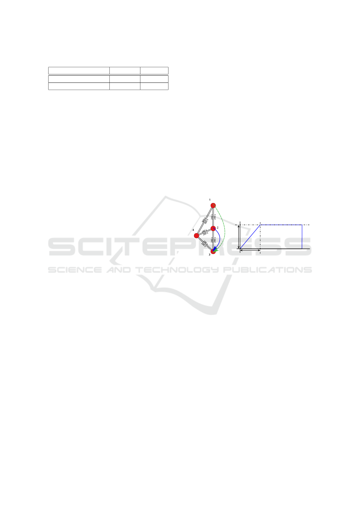
Table 1: Cost and congested ﬂow: Road Network A.

capacity constraints strict relaxed

Steady-state approach infeasible 14 (6/4)

Dynamic approach 15 15 (0/0)

sulting graph is G

= (V

), where V

= V

∪V

and E

= E

∪ E

. The trafﬁc ﬂows over time are

deﬁned analogically as steady-state ﬂows, the differ-

ence is that these are deﬁned on the time-expanded

graph G

. Finally, we deﬁne the solution of the on-

demand ﬂeet routing over time on road graph G to be

the solution of the steady-state on-demand ﬂeet rout-

ing over the time-expanded graph G

. The described

approach is later referred as the dynamic approach.

6.1 Dynamic Approach Solution

The model of ﬂows over time, in contrast with the

steady-state approach, considers both previous and

predicted future ﬂows. Fig. 2b shows the optimal so-

lution of the Problem 1 with time provided by the dy-

namic approach. The steady-state approach ignores

previous ﬂows, so when the partial ﬂows are put to-

gether in time the resulting ﬂows can exceed the road

capacity. We refer to such a solution as being infea-

sible. We already showed that for Road Networks A,

the solution of the steady-state approach is infeasible.

We compare the solution quality of the considered

approaches on the Road Network A in Table 1. We

compare the approaches in two settings: 1) we con-

sider problems strictly as deﬁned, 2) we relax the road

capacity constraints if no other feasible solution ex-

ists. In the strict setting, we can conﬁrm that the basic

steady-state approach that ignores previous ﬂows is

infeasible. The dynamic approach ﬁnds the optimal

feasible solution in the both settings.

If we relax the capacity constraints in the case no

feasible solution is found, we can observe lower costs

in steady-state approach, but the rate of vehicle ﬂows

may exceed the capacity constraints of the road links.

The exceeded capacity is described in brackets in the

form (F/C) where F is a the sum of ﬂows on the

edges with exceeded capacity and the C is a capacity

constraint over such edges. The values reveal by how

much are the capacities exceeded, which also hints on

the severity of congestion that would appear in prac-

tice. In Table 1 we observe that the steady-state ap-

proach can assign ﬂows that consume up to 150% of

the road capacity.

7 SIMULATION EVALUATION

In this section, we will evaluate the performance of

the proposed ﬂeet routing approach in simulation. For

evaluation, we use an abstract model of a part of a city

highway network shown in Fig. 3a. The road network

connects the city center (N. 2) to three peripheries (N.

1, 3, 4) of a small metropolitan area. We study the

interaction of a through-trafﬁc demand ﬂow (N. 1 →

N. 3) with a local-trafﬁc demand ﬂow (N. 2 → N. 3)

during morning trafﬁc peak. The intensity of trans-

portation demand in each of these demand ﬂows in-

creases in time up to a saturation level according to a

trapezoid impulse function depicted in Fig. 3b. The

shape of the demand ”impulse” is controlled by tau

and peak parameters. The former represents the time

to reach full saturation, measured in seconds. The lat-

ter represents the intensity at full saturation relative to

the free-ﬂow capacity of a road segment.

(a)

peak

tau

time 2h

(b)

Figure 3: Test Scenario. Road network and the two demand

ﬂows (left) and the shape of demand ”impulse” (right).

7.1 Congestion Model

The travel velocity on the individual edges is mod-

eled as density-dependent. We use an empirical

two-regime link delay model for highway segments.

The vehicles are able to drive at free-ﬂow speed un-

til the vehicle density at the link exceeds so-called

free-ﬂow capacity. In our case, the free-ﬂow den-

sity is 20 veh./km, which corresponds to the ﬂow of

0.55 veh./sec. at 100 km/h. At this point, the traf-

ﬁc enters so-called bound ﬂow regime and the ve-

hicles start decreasing their velocity. One of the

crucial empirical observations made by transporta-

tion researchers is that, initially, the density of ve-

hicles increases slightly faster then their speed re-

duces and thus the vehicle ﬂow is typically observed

to increase until the density reaches so-called criti-

cal capacity. The critical capacity in our model corre-

sponds roughly to the density of 25 veh./km and ﬂow

of 0.56 veh./sec. at 80 km/h. After the critical capac-

ity has been exceeded, both the velocity and the ﬂow

ICAART 2021 - 13th International Conference on Agents and Artiﬁcial Intelligence

912

of trafﬁc start rapidly declining. At this point, the sys-

tem enters an unstable regime with self-reinforcing

feedback loop that eventually leads to build-up of

standstill or slowly moving queues.

7.2 Experiment Setup

We compare the performance of three ﬂeet-routing

strategies: In shortest-path approach, all vehicles are

routed along the shortest path from the origin of each

demand request to its destination. In steady-state ap-

proach, we compute the routes by sequentially solv-

ing the steady-state formulation as described in Sec-

tion 5.2. In dynamic approach, we compute the routes

by solving the ﬂows over time formulation as de-

scribed in Section 6. The capacity constraint of each

road segment is set to correspond to free-ﬂow capac-

ity of that edge, i.e, it is set to 0.55 veh./sec. In reality,

the edge free-ﬂow capacities might be too restrictive

for high demand, and cause the approaches to fail to

provide a feasible solution. For such cases, the capac-

ity constraints are modeled as elastic constraints. The

capacity can be exceeded for additional penalty that

is linear in the capacity excess and the link free-ﬂow

traversal time. The penalty enforces that the capacity

is exceeded only if no other feasible solution exists.

We generate two hours of through-trafﬁc and

local-trafﬁc transportation demand discretized to

2 min. timesteps following trapezoidal shape with dif-

ferent combinations of tau and peak parameters. In

particular, we create the combination such that tau

takes values 20 min, 30 min, 45 min, and 60 min and

peak takes values 0.5, 0.55, .. ., 1.25. This will al-

low us to study how does the dynamism and the scale

of the demand affect the performance of the individ-

ual approaches. Then we let each approach to gener-

ate routes for all the vehicles serving the transporta-

tion demand. Finally, we simulate the movement of

individual vehicles in the multi-agent trafﬁc simula-

tor Agentpolis employing the congestion model de-

scribed in the previous section and record the travel

delay of each vehicle.

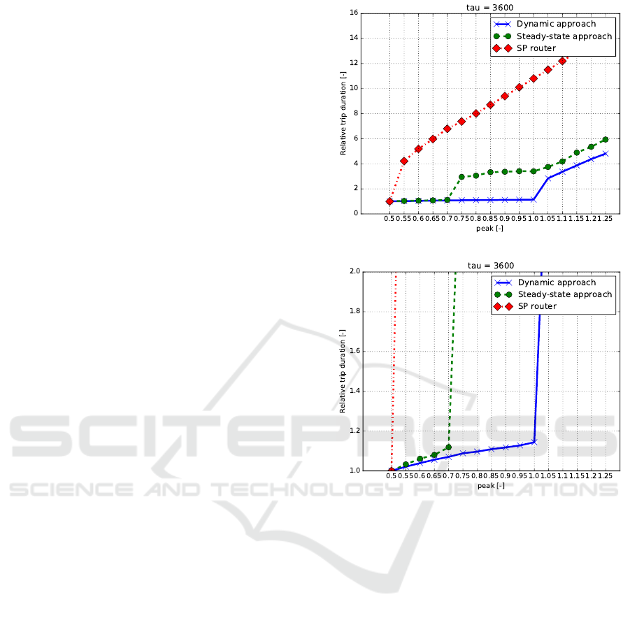
7.2.1 Results

The average travel prolongation achieved by the three

compared methods as a function of peak parameter is

shown in Fig. 4 for slowly (1 h to saturation) evolving

demand. To correctly interpret the results, it is useful

to observe that there are two key thresholds for peak

parameter. Firstly, since we are only working with

two demand ﬂows, for peak ≤ 0.5, it is impossible to

exceed the link capacity (unless some vehicle travel

along some segment multiple times) and thus all three

approaches maintain zero prolongation. On the other

(a) Overall view

(b) Zoomed view on prolongation values for under-capacity

ﬂows

Figure 4: Average Travel Prolongation vs. peak, tau = 60

min.

hand, for peak > 1, the link capacities will be neces-

sarily exceeded by any routing policy. Thus, we are

interested in the ability of the three routing policies to

maintain reasonable delay in between these two ex-

tremes.

As we can see, the congestion-unaware shortest

path policy routes both demand ﬂows through the cen-

ter and thus the trafﬁc on link (2,3) quickly exceeds

the critical intensity and enters the unstable, highly

congested regime, resulting in extremely high travel

delays. The steady-state approach initially serves the

through-trafﬁc demand ﬂow by two vehicle ﬂows, one

going through the center, the other one routed through

the periphery. Since a portion of the vehicles travel

via a route that is 25 % longer than the shortest route,

the average travel prolongation is slightly increased.

The fact that steady-state approach does not account

for future changes in demand results in excess trafﬁc

On-demand Robotic Fleet Routing in Capacitated Networks with Time-varying Transportation Demand

913

on link (2, 3). This undesirable excess ﬂow is larger

for larger values of peak and for faster change in de-

mand, i.e, for smaller values of tau. The ﬂow eventu-

ally grows large enough to exceed the critical capac-

ity, leading again to collapse of the trafﬁc ﬂow and

subsequently to signiﬁcant travel delays. Since the

trafﬁc collapses only for the through-ﬂow routed via

the city center and the vehicles driving via the periph-

ery remain traveling at free-ﬂow speed, the average

prolongation remains smaller than the average prolon-

gation for the shortest path strategy.

The dynamic approach successfully accounts for

anticipated future demand by preemptively routing

part of the through-ﬂow via the periphery. Although

this results in up to 1.2x travel time prolongation, the

algorithm maintained sub-critical ﬂows in the system

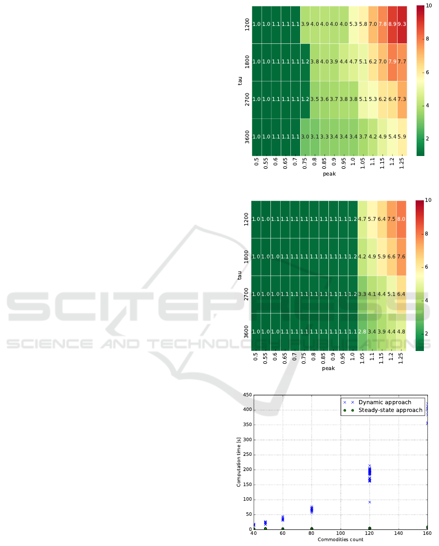
for all peak values < 1.0. For completeness, the com-

parison of average travel delay for steady-state and

dynamic approach for all combinations of values for

tau and peak parameters are depicted in Fig. 5b. The

same phenomena can be observed.

These results suggest that system optimal ﬂeet

routing that explicitly addresses time-varying demand

has a potential to signiﬁcantly increase the amount

of transportation demand that can be efﬁciently trans-

ported through existing road infrastructures. Indeed,

compared to the shortest path approach, the proposed

technique can be used to service twice as many trans-

portation request in the same road network with-

out worsening the congestion. In comparison to the

steady-state approach, the dynamic method is capable

of servicing 42 % extra demand (1.0 vs. 0.7) through

the same road network.

The dynamic approach results in a large linear

program that is computationally demanding to solve

optimally using general solution techniques as shown

in Fig. 5c. The linear program can have up to T · M ·

(|E|+M + |V |) variables and T ·M ·|V | + M

+|E|·T

constraints. The most limiting factor in the sense of

the scalability is M - the number of demand ﬂows (i.e.,

commodities). Recall that a demand ﬂow is an aggre-

gation of requests that have the same origin, destina-

tion, the earliest pick-up and the latest drop-off time.

In the worst case the M is in order of V

·T even under

the additional assumption that the latest drop-off time

is dependent on the three other demand ﬂow parame-

ters. Thus, the number of constraints may, in the worst

case, grow with |V |

, which makes this approach im-

practical for detailed model of large metropolitan net-

works that may contain tens or hundreds of thousands

of vertices. Solving large-scale instances will thus

likely require application of more advanced solution

techniques. The results of (Schaefer et al., 2019) on

the steady state problem variant indicate that Dantzig-

(a)

(b)

(c)

Figure 5: Average delay for combinations of tau and peak

for the steady-state (a) and the dynamic (b) approach. Scal-

ability (c): computation time for 2 h demand, the commodi-

ties count is varied by adapting the timestep.

ICAART 2021 - 13th International Conference on Agents and Artiﬁcial Intelligence

914

Wolf decomposition (Dantzig and Wolfe, 1960) could

be also employed to solve larger scale instances of our

problem with time-varying demand.

8 CONCLUSION

To conclude, in this paper, we identiﬁed the prac-

tical limitations of steady-state approach to solve

on-demand ﬂeet routing when the demand is time-

varying. We proposed an alternative approach that

explicitly models the evolution of system in time.

We implemented both steady-state and dynamic ap-

proaches and compared them on the simpliﬁed, but

characteristic illustrative example. While the steady-

state approach fails to ﬁnd a solution or generate

routes that exceed route link capacities by up to 50 %,

the proposed approach is able to solve such instances

without exceeding the road link capacities. Conse-

quently, the simulation experiments with the conges-

tion model reveal that the proposed approach that uses

the ﬂows over time model outperforms the steady-

state approach in presence of the time-varying de-

mand. The dynamic solution can transfer 42% more

demand in the congestion-free regime than the steady-

state approach on the same illustrative road network.

The proposed model that explicitly models time is

larger and generally harder to analyze and compute

than the steady-state model. Therefore, in future

work, we will study the applicability of specialized

solution techniques for large-scale linear programs,

e.g. the applicability of Dantzig-Wolfe decomposi-

tion method as applied in (Schaefer et al., 2019), to

improve the scalability of the proposed approach.

ACKNOWLEDGEMENTS

The authors acknowledge the support

of the OP VVV MEYS funded project

CZ.02.1.01/0.0/0.0/16 019/0000765 ”Research

Center for Informatics” and TACR NCK project

T N01000026 ”Josef Bozek National Center of

Competence for Surface Vehicles”.

REFERENCES

Berbeglia, G., Cordeau, J.-F., Gribkovskaia, I., and Laporte,

G. (2007). Rejoinder on: Static pickup and delivery

problems: a classiﬁcation scheme and survey. TOP,

15(1):45–47.

Dantzig, G. B. and Wolfe, P. (1960). Decomposition Prin-

ciple for Linear Programs. Operations Research,

8(1):101–111.

Even, S., Itai, A., and Shamir, A. (1975). On the complexity

of time table and multi-commodity ﬂow problems. In

Foundations of Computer Science, 1975., 16th Annual

Symposium on, pages 184–193. IEEE.

Fiedler, D.,

ap, M., and

Certick

y, M. (2017). Im-

pact of mobility-on-demand on trafﬁc congestion:

Simulation-based study. In 2017 IEEE 20th Interna-

tional Conference on Intelligent Transportation Sys-

tems (ITSC), pages 1–6. IEEE.

Ford, L. R. and Fulkerson, D. R. (1958). Constructing Max-

imal Dynamic Flows from Static Flows. Operations

Research, 6(3):419–433.

Frederickson, G. N., Hecht, M. S., and Kim, C. E. (1976).

Approximation algorithms for some routing problems.

In 17th Annual Symposium on Foundations of Com-

puter Science (sfcs 1976), pages 216–227.

Pillac, V., Gendreau, M., Gu

eret, C., and Medaglia, A. L.

(2013). A review of dynamic vehicle routing prob-

lems. European Journal of Operational Research,

225(1):1–11.

Rossi, F., Zhang, R., and Pavone, M. (2016). Congestion-

aware randomized routing in autonomous

mobility-on-demand systems. arXiv preprint

arXiv:1609.02546.

Schaefer, M.,

ap, M., Mrkos, J., and Vok

ınek, J. (2019).

Routing a ﬂeet of automated vehicles in a capacitated

transportation network. In 2019 IEEE/RSJ Interna-

tional Conference on Intelligent Robots and Systems

(IROS), pages 8223–8229.

Solovey, K., Salazar, M., and Pavone, M. (2019). Scal-

able and congestion-aware routing for autonomous

mobility-on-demand via frank-wolfe optimization. In

Robotics: Science and Systems, Freiburg im Breisgau,

Germany.

Spieser, K., Treleaven, K., Zhang, R., Frazzoli, E., Mor-

ton, D., and Pavone, M. (2014). Toward a Systematic

Approach to the Design and Evaluation of Automated

Mobility-on-Demand Systems: A Case Study in Sin-

gapore. In Road Vehicle Automation, pages 229–245.

Springer.

The Technical Administration of Roads of the City of

Prague (2020). Prague transportation yearbook

2019. http://www.tsk-praha.cz/static/udi-rocenka-

2019-en.pdf. Accessed: Nov 26, 2020.

Wollenstein-Betech, S., Houshmand, A., Salazar, M.,

Pavone, M., Cassandras, C. G., and Paschalidis, I. C.

(2020). Congestion-aware routing and rebalancing

of autonomous mobility-on-demand systems in mixed

trafﬁc. In Proc. IEEE Int. Conf. on Intelligent Trans-

portation Systems, Rhodes, Greece. In press.

Zhang, R., Rossi, F., and Pavone, M. (2016a). Routing

autonomous vehicles in congested transportation net-

works: Structural properties and coordination algo-

rithms. In Robotics: Science and Systems XII, Uni-

versity of Michigan, Ann Arbor, Michigan, USA, June

18 - June 22, 2016.

Zhang, R., Rossi, F., and Pavone, M. (2016b). Routing Au-

tonomous Vehicles in Congested Transportation Net-

works: Structural Properties and Coordination Algo-

rithms. In Robotics: Science and Systems XII, vol-

ume 42, pages 1427–1442. Robotics: Science and

Systems Foundation.

On-demand Robotic Fleet Routing in Capacitated Networks with Time-varying Transportation Demand

915