Clustering-based Sequential Feature Selection Approach for High
Dimensional Data Classification
M. Alimoussa
1,2
, A. Porebski
1
, N. Vandenbroucke
1
, R. Oulad Haj Thami
2
and S. El Fkihi
2
1
Univ. Littoral C
ˆ
ote d’Opale, UR 4491, LISIC, Laboratoire d’Informatique Signal et Image de la C
ˆ
ote d’Opale,
F-62100 Calais, France
2
Univ. Mohammed V, ADMIR, Advanced Digital Entreprise Modeling and Information Retrieval Laboratory,
Keywords:
Dimensionality Reduction, Feature Selection, Color Texture Classification.
Abstract:
Feature selection has become the focus of many research applications specially when datasets tend to be
huge. Recently, approaches that use feature clustering techniques have gained much attention for their ability
to improve the selection process. In this paper, we propose a clustering-based sequential feature selection
approach based on a three step filter model. First, irrelevant features are removed. Then, an automatic feature
clustering algorithm is applied in order to divide the feature set into a number of clusters in which features
are redundant or correlated. Finally, one feature is sequentially selected per group. Two experiments are
conducted, the first one using six real wold numerical data and the second one using features extracted from
three color texture image datasets. Compared to seven feature selection algorithms, the obtained results show
the effectiveness and the efficiency of our approach.
1 INTRODUCTION
Feature dimensionality reduction has been success-
fully applied to diverse fields of machine learning
such as data classification (Chandrashekar and Sahin,
2014; Harris and Niekerk, 2018). Classification is the
process of predicting the class of input data to one
of a set of categories. When the data is represented
in a high-dimensional feature space, dimensionality
reduction is required to improve the performance of
the classifier. It is achieved either by feature extrac-
tion or by feature selection schemes during a learning
process. Feature extraction techniques reduce the fea-
ture space dimensionality by transforming the origi-
nal feature space into a new reduced size feature set.
However, this transformation leads to the change of
the semantic and the explainability of the original fea-
ture space. Moreover, such a transformation requires
the computation of the initial feature set to obtain the
new reduced feature space, which could be time con-
suming. The goal of feature selection is to find a rele-
vant subset from an original feature space that can, de-
pending on an evaluation function, improve the over-
all performance of a classification algorithm. Indeed,
performing feature selection can not only improve the
accuracy, the feasibility and the efficiency of a clas-
sification algorithm, but also reduces the complex-
ity, the memory storage and the computation time re-
quired to achieve it while providing a better under-
standing of the data (Hsu et al., 2011; Chandrashekar
and Sahin, 2014).
A feature selection process can be achieved by
two main models named ”filter” and ”wrapper” (Das,
2001). Filter models deploy statistical measures
to evaluate features or subsets of features, whereas
wrapper models compute the accuracy reached with
a particular classifier in order to guide the search for
determining the most discriminating feature subset.
Other techniques, called hybrid or embedded mod-
els, combine both filter and wrapper approaches (Hsu
et al., 2011). On the one hand, wrapper models tend to
achieve better results than filter ones, but suffer from
a high computational cost since they depend to a clas-
sifier (Hall, 2000; Yu and Liu, 2003). On the other
hand, filter models are simple to design, classifier in-
dependent and faster. This makes filter models often
chosen over the wrapper ones, particularly when the
number of features becomes very high. In this paper,
we propose a filter approach to address the problem of
feature selection in the case of high dimensional data.
A feature selection algorithm can be performed
on a training dataset either by feature ranking or by
122
Alimoussa, M., Porebski, A., Vandenbroucke, N., Thami, R. and El Fkihi, S.
Clustering-based Sequential Feature Selection Approach for High Dimensional Data Classification.
DOI: 10.5220/0010259501220132
In Proceedings of the 16th International Joint Conference on Computer Vision, Imaging and Computer Graphics Theory and Applications (VISIGRAPP 2021) - Volume 4: VISAPP, pages
122-132
ISBN: 978-989-758-488-6
Copyright
c
 2021 by SCITEPRESS – Science and Technology Publications, Lda. All rights reserved

feature subset search. Feature ranking algorithms in-
dividually rank features in order to select the most
discriminating ones. Therefore, they are fast and
easy to apply. However, it has been shown that the
combination of individually relevant features does not
necessary yield to a high classification performance
(Hanchuan Peng et al., 2005). This is mainly due to
the non consideration of the interactions and the re-
dundancy that may exist between features. Feature
subset search generally follows 4 stages ; a) the gener-
ation of feature subsets, b) the evaluation of the gen-
erated feature subsets, c) the stopping of the search
and d) the validation (Yu and Liu, 2003). The sub-
set generation stage is defined by a search strategy,
which can be either exhaustive, sequential or random.
The generated subset is evaluated in the second stage
by means of an evaluation function which is the ac-
curacy of a classifier in the case of wrapper models
and a statistical measure in the case of a filter one.
The search stops when a stopping criterion is satisfied
and the subset with the optimal value of the evalu-
ation function is returned with its dimensionality as
the most discriminating feature subset. Then, it can
be validated through a specific validation dataset.
When dealing with high dimensional data
(datasets with hundred or thousands of features),
many feature selection approaches can successfully
remove irrelevant features but fail to pull redundant
ones out (Kira and Rendell, 1992; Song et al., 2013;
Hall, 2000). To overcome this problem, several fea-
ture selection algorithms that use feature clustering
were proposed in the last decades in both supervised
and unsupervised context (Song et al., 2013; Zhu
et al., 2019; Mitra et al., 2002; Harris and Niekerk,
2018; Li et al., 2011; Zhu and Yang, 2013; Yousef
et al., 2007). In this paper, we focus on clustering-
based feature selection approaches in a supervised
context. The goal of these approaches is to divide
the initial feature space into a set of groups called
clusters. Generally, dependency measures are used as
clustering algorithm metrics, which makes features of
the same group considered as redundant. This leads to
the selection of one feature to represent each cluster.
The resulting feature subset is considered to be rele-
vant and non redundant (Zhu et al., 2019). Clustering-
based feature selection algorithms can outperform the
traditional feature selection methods by reducing the
redundancy, reaching a high accuracy and, in some
cases, reducing the calculation time. Even though
they have recently gained much attention, their num-
ber is still relatively limited and need parameters to
be adjusted (Song et al., 2013). In this paper, we
propose an original clustering-based sequential fea-
ture selection approach that uses a filter model for the
classification of high dimensional data. In a first time,
a feature clustering is automatically defined using a
separability measure and used, in a second time, by a
sequential search algorithm in order to obtain a rele-
vant and non redundant feature subset: once a feature
is selected, features of the same cluster are removed
and thus not considered in the next steps of the selec-
tion process. This approach significantly speeds this
process up since large number of redundant features
are eliminated at each step. In our knowledge, the
proposed approach is the only one which applies a fil-
ter model-based sequential feature selection scheme
to all the features belonging to different clusters so
that only one feature per cluster is selected at each
step before removing these clusters. A second orig-
inality of our approach is that the feature clustering
stage is fully automatic and does not required any pa-
rameters to be adjusted.
The proposed approach is well suited to address
the color texture classification problems. In these
problems, color textures are often represented by the
combination of different descriptors computed from
images coded in multiple color spaces(Alimoussa
et al., 2019). This leads to a massive amount of tex-
ture features (in the order of thousands). Since most
of these features are considered either irrelevant or re-
dundant features, removing them can help to improve
the classification process, in terms of accuracy and
computational time. Applying a feature clustering-
based selection approach on image features aims to
group redundant features into the same clusters so that
only one relevant feature can be chosen per cluster
in order to build a discriminating feature space of re-
duced dimensionality.
The rest of this paper is organized as follows. Sec-
tion 2 presents a state of the art of clustering-based
feature selection approaches in the supervised con-
text. Then the proposed approach is detailed in sec-
tion 3. In section 4, two experiments are conducted to
validate our approach: the first one is carried out us-
ing six real world numerical datasets, and the second
one using features extracted from three color texture
image datasets. Finally, section 5 holds the conclu-
sion of the paper.
2 RELATED WORKS
The clustering-based feature selection approaches can
be divided into two categories: those that use a subset
search algorithm and those that consider a simple fea-
ture ranking. Figure 1 illustrates the state of the art of
these approaches that are detailed in the next sections.
Clustering-based Sequential Feature Selection Approach for High Dimensional Data Classification
123

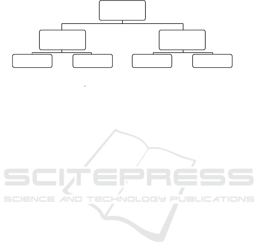
Clustering-based
feature selection
Subset search
algorithms
Filter
Wrapper
CSFS (Proposed) - RCE
(Yousef et al., 2007)
- AP SFS
(Zhu and Yang, 2013)
- KA
(Krier et al., 2007)
Ranking algorithms
Filter
Wrapper
- FCR
MI
(Harris and Niekerk, 2018)
- FAST
(Song et al., 2013)
- SSF
(Cov
˜
oes and Hruschka, 2011)
- FCR
NB
(Harris and Niekerk, 2018)
- CSF
(Li et al., 2011)
Figure 1: State of the art of the clustering-based feature selection methods.
2.1 Clustering-based Feature Ranking
Algorithms
Traditionally, feature selection using a feature ranking
algorithm is focused on removing irrelevant features,
neglecting the possible redundancy between relevant
ones (Song et al., 2013). This is the reason why some
approaches prefer to use a feature clustering analy-
sis before ranking features. Indeed, most clustering-
based feature ranking algorithms develop a two stage
procedure. First, the feature space is divided into a
number of groups by means of a clustering algorithm.
Then, feature in each cluster are ranked in order to
select representative features of each group.
A three step method called Feature Clustering and
Ranking (FCR) was developed in (Harris and Niek-
erk, 2018). First, a feature clustering is performed
using the affinity propagation algorithm and the cor-
relation coefficient as similarity measure. Then, each
cluster is ranked by using a cluster score. This clus-
ter score is defined by the median of the feature rele-
vance value in the cluster. A single feature from each
of the best clusters is finally selected. Two criteria are
tested for measuring the feature relevance: the mu-
tual information between the class labels and the fea-
tures leading to the FCR
MI
filter model, and the ac-
curacy reached with a Naive Bayes classifier defining
the FCR
NB
wrapper model.
Song et al. proposed another clustering-based fea-
ture ranking algorithm called FAST, which uses a
filter model (Song et al., 2013). At the first stage,
features are divided into clusters by using a cluster-
ing method based on graph-theoretic. Then, for each
group, the feature the most correlated to the class la-
bels is selected to form the final feature subset.
Li et al. applied a wrapper model with the Support
Vector Machine (SVM) classifier (Li et al., 2011).
This approach, called CSF, starts by clustering fea-
tures using the correlation-based affinity propagation
algorithm. Then, features of each cluster are ranked
according to their sensitivity using SVM. The most
class sensitive feature of each cluster is retained to
form the final feature subset.
Cov
˜
oes et al. proposed the Simplified Silhouette
Filter (SSF) (Cov
˜
oes and Hruschka, 2011). The ap-
proach uses a simplified version of the silhouette co-
efficient to automatically cluster features using the K-
medoids clustering algorithm. For this purpose, dif-
ferent values of the parameter K are tested. Then they
propose two ways to select features from each cluster.
The first one selects two features from each cluster;
the most correlated feature and the feature the least
correlated to the other features of the same cluster.
The second one selects only the feature the most cor-
related to the other features of the same cluster. Based
on the average classification error, SSF obtained bet-
ter results considering the selection of two features
from each cluster rather than one.
2.2 Clustering-based Feature Subset
Search Algorithms
Clustering-based feature subset selection can be done
following three strategies:
(i) As a pre-processing stage that comes before the
search. Krier et al. has developed such an approach
that we call KA (Krier et al., 2007). The algorithm
clusters features into an appropriate number of groups
using feature consecutive clustering algorithm. Then,
considering the mutual information, only one feature
from each group is retained to form a feature subset
which will be the input of a Radial basis function net-
VISAPP 2021 - 16th International Conference on Computer Vision Theory and Applications
124

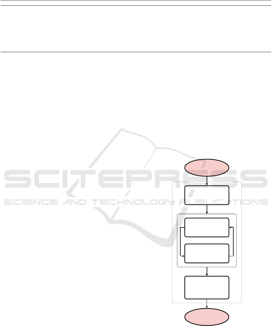
Table 1: State of the art of the clustering-based feature selection approaches.
Approach Used clustering algorithm Selecting type Model Evaluation metric
KA (Krier et al., 2007) Feature Consecutive Clustering Feature subset search Wrapper RBFN and Mutual Information
FCR
MI
(Harris and Niekerk, 2018) Affinity Propagation Feature ranking Filter Mutual Information
FCR
NB
(Harris and Niekerk, 2018) Affinity Propagation Feature ranking Wrapper Naive Bayes
RCE (Yousef et al., 2007) K-means Feature subset search Wrapper SVM
AP-SFS (Zhu and Yang, 2013) Affinity Propagation Feature subset search Wrapper KNN, Naive Bayes and LDA
FAST (Song et al., 2013) Graph-theoretic based approach Feature ranking Filter Symmetrical Uncertainty
SSF (Cov
˜
oes and Hruschka, 2011) K-medoids Feature ranking Filter Maximal Information Compression
CSF (Li et al., 2011) Affinity Propagation Feature ranking Wrapper SVM
CSFS (proposed) Long Correlation Feature subset clustering Filter Trace criterion
work (RBFN) based sequential feature selection algo-
rithm.
(ii) Combined with the search strategy. For ex-
ample, the Recursive Cluster Elimination (RCE) ap-
proach uses the K-means to cluster features into a
predefined number of groups and then evaluates each
group of features using the SVM classifier (Yousef
et al., 2007). Low performance feature groups are re-
moved, the remaining feature groups are merged and
the whole process is repeated.
(iii) As a search strategy alternative. An exam-
ple of this technique, called AP-SFS, is proposed by
Zhu and Yang (Zhu and Yang, 2013). This approach
clusters features using a modified affinity propagation
algorithm and then applies a sequential search in each
group. Selected features from each group are merged
to form the final selected feature subset.
All the clustering-based feature ranking and sub-
set search feature selection approaches presented in
Figure 1 and described in this section are summarized
in Table 1. For each method, the used clustering al-
gorithm, the selection type, the model (filter, wrapper
or hybrid) and the evaluation function are described.
Different from these approaches, the originality of the
approach proposed in this paper is that it uses a filter
model-based feature subset search algorithm applied
to all the features belonging to different automatically
determined clusters and so that only one feature per
cluster is selected at each step before removing these
clusters.
3 PROPOSED METHOD
The proposed Clustering-based Sequential Feature
Selection (CSFS) approach consists of three stages as
shown in Figure 2.
(1) First, irrelevant features are removed. For this
purpose, the correlation is measured between each
feature and the class labels. We assume that the
less a feature is correlated with the class labels of
the samples, the lower its ability to discriminate be-
tween classes is. Here, 5% of low class-correlation
features are pulled out of the initial feature set (Bins
and Draper, 2001) (see section 3.1).
(2) A dependency graph-based clustering method
called Long Dependency is then considered to cluster
the feature space. The method uses a correlation co-
efficient whose threshold is automatically determined
by evaluating the feature clustering with a feature sep-
arability measure (see section 3.2).
(3) Finally, a Sequential Forward Selection (SFS)
approach, based on a filter model, is applied to the
initial feature space. Once a feature is selected, fea-
tures belonging to the same cluster are removed and
thus not considered in the next steps. As a conse-
quence, the number of candidate features dramatically
decreases at each step (see section 3.3).
Initial feature
set
Irrelevant feature
removal
Correlation-based
feature clustering
Clustering
evaluation
Sequential
feature
selection (SFS)
Selected
feature subset
(1)
(2)
(3)
Figure 2: Flowchart of the proposed CSFS approach.
The dependency measure used in the first and sec-
ond stage of our system is defined by the simple and
linear Pearson correlation.
Clustering-based Sequential Feature Selection Approach for High Dimensional Data Classification
125

3.1 Correlation Measure
The Pearson correlation ρ between two sample vec-
tors X =

x
1
. . . x
n

and Y =

y
1
. . . y
n

of n values
is defined by the following equation:
ρ(X, Y ) =
∑
n
i=1
(x
i
− ¯x)(y
i
− ¯y)
p
∑
n
i=1
(x
i
− ¯x)
2
p
∑
n
i=1
(y
i
− ¯y)
2
, (1)
where ¯x is the mean of X and ¯y is the mean of Y . If X
and Y are totally dependent, the value of ρ tends to its
limits 1 or -1, and if they are completely independent,
ρ is close to zero.
For the first stage of our approach, X is the sam-
ple vector X
k
of a feature F
k
that contains the feature
values of the n considered data and Y is a vector that
represents the class labels of those data. For the sec-
ond stage, X and Y are two sample vectors X
k
and X
l
of features F
k
and F
l
respectively that contain the fea-
ture values of the n data.
3.2 Dependency Measure based
Clustering Strategy
To help understand the second stage of the proposed
clustering-based algorithm, let us consider a graph
where nodes are the considered features (see Figure
3). Two features (i.e. nodes) are linked if they are
correlated (ie. the absolute value of the correlation
between them, defined by Equation (1) is higher than
a threshold). We consider the features which are in-
directly (via other features) connected to be ”long de-
pendent”. Dependent and long dependent features are
put into the same feature cluster.
Figure 3: Example of correlated features.
We define the concept of Long Dependency be-
tween two features as follows:
Let F be the candidate feature set. Two features
F
k
and F
l
belonging to F are considered to be long de-
pendent iff ∃F
m
∈ F , F
k
is dependent to F
m
and F
l
is
dependent to F
m
. We propose to illustrate our cluster-
ing strategy thanks to an example with a feature set of
ten features: F = (F
1
, F
2
, F
3
, F
4
, F
5
, F
6
, F
7
, F
8
, F
9
, F
10
).
Giving a correlation threshold, let us consider the cor-
relation between features shown in Figure 3 where
correlated features are attached via a line.
From the correlation graph presented in Figure 3,
we conclude the clustering result presented in Figure
4. Note that F
1
and F
9
, and F
5
and F
6
are long depen-
dent and therefore they belong to the same cluster.
Figure 4: Resulting clustering.
Let us note that the higher the correlation thresh-
old is, the less the number of initial links between fea-
tures is, the less the number of correlated and also
long correlated features is, and therefore the more the
number of clusters is.
The correlation threshold is the only one param-
eter of the clustering algorithm. As many clustering
algorithms such as K-means and affinity propagation,
the parameters directly impact the clustering result.
Choosing the right parameters is a very crucial issue.
That is the reason why we have chosen to automate
this choice. This automatic setting is a key point of
our approach since parameters generally have to be
adjusted by the user. This operation is done by vary-
ing the correlation coefficient threshold and then eval-
uating the clustering quality. This evaluation is per-
formed using the Trace separability measure defined
in Equation (2) which is to be maximized.
3.3 Clustering-based Sequential
Feature Selection
Since features of a same cluster are considered as re-
dundant, only one feature per cluster is considered.
The main originality of our approach is to sequen-
tially select only one feature from each cluster by a
filter model.
The proposed method, CSFS, uses feature clus-
tering combined with the search strategy. Following
a forward sequential strategy, the feature selection al-
gorithm selects, at each step, a feature from the candi-
date feature space depending on the value of the eval-
uation function. Once the feature is selected, the clus-
ter in which this feature belongs is removed to define
the remaining candidate feature set that will be evalu-
ated at the next step. This feature cluster removal aims
to achieve two goals. First, feature redundancy is re-
duced and only relevant and non redundant features
are selected. Second, compared to a classical sequen-
tial feature selection method, the process is speed up
since several features are removed at each step.
Since a correlation-type measure was used in the
first and second step, and in order to achieve a
multi-criterion approach, we have chosen to use, for
this step of our approach, a distance-based criterion
VISAPP 2021 - 16th International Conference on Computer Vision Theory and Applications
126

to evaluate the relevance of each candidate feature
space. Correlation-type measures and distance-based
criteria are indeed complement each other, which al-
lows to improve the efficiency of the selection pro-
cess (Porebski et al., 2010). To define the considered
distance-based criterion, called Trace, let us introduce
the following notations:
Let X, be a n × p matrix that represents a
database of n samples characterized by p variables
(features). Each of the p columns of the matrix
X is the n-dimensional sample vector X
k
that repre-
sent a feature F
k
. Each of the n rows of the ma-
trix X is the p-dimensional feature vector X
i, j
=
h
x
i, j
1
. . . x
i, j
k
. . . x
i, j
p
i
of the i
th
sample (i = 1, . . . , N
j
w
)
of the j
th
class ( j = 1, . . . , N
c
) where x
i, j
k
is the k
th
fea-
ture value of this sample, N
c
is the number of classes
and N
j
w
is the number of samples for each class j.
Let M
j
=
h
m
j
1
. . . m
j
k
. . . m
j
p
i
, be the p-dimensional
mean feature vector on the N
j
w
samples of the class
j, with M
j
k
, the mean of the feature F
k
over the sam-
ples in the class j, and M = [m
1
. . . m
k
. . . m
p
], be the
p-dimensional mean feature vector on the n samples,
with M
k
, the mean of the feature F
k
over all samples.
For a feature subset F , the Trace criterion is given
by:
Tr(F ) = trace(((M
W
+ M
B
)
−1
) ×M
B
), (2)
where trace(A) is the trace of the matrix A, M
B
is the
between-class matrix defined by the following equa-
tion:
M
B
=
1
N
c
N
c
∑
j=1
(M
j
− M)(M
j
− M)
T
, (3)
and M
W
is the within-class matrix, defined as fol-
lows:
M
W
=
1
N
c
× N
j
w
N
c
∑
j=1
N
j
w
∑
i=1
(X
i, j
− M
j
)(X
i, j
− M
j
)
T
. (4)
The search stops when a local maximum value of
the Trace separability criterion is observed or when a
maximum number D of iterations is achieved.
The algorithm of the proposed approach is define
in Algorithm 1. In this algorithm, the three steps of
the proposed approach are detailed.
In Step 1, a list called List of features sorted by
their correlation value with the class labels is gener-
ated. Only a percentage of features most correlated
with the class labels are kept in the initial feature set.
In Step 2, the remaining features are clustered us-
ing the Long dependency clustering algorithm defined
Algorithm 1: The proposed clustering-based sequential fea-
ture selection.
Input
S = {X
k
k = 1, . . . , p}, the feature set where p is
the number of features
L, the class label set of the n samples
D, the maximum dimension
Output
(C
1
, . . . , C
a
, . . . , C
b
), the set of feature clusters
where each cluster C
a
(a = 1, . . . , b) contains n
a
fea-
tures (n
a
≥ 1)
S
t
= {Y
l
l = 1, ·· · , t}, the selected feature set
where t is the number of selected features (1 ≤ t ≤
D)
Step 1 : Low class-correlation features removal
List = {{k, ρ(X
k
, L)} k = 1, . . . , p}
List = sort(List, ’descending’)
S = {X
k
k = List(1, 1). . . List(percentage×
p, 1)}
Step 2 : Automatic feature clustering
threshold = argmax Tr((LD(S , thresholds))
(C
1
, . . . , C
a
, . . . , C
b
) = LD(S , threshold)
Step 3 : Clustering-based sequential feature
selection
S
0
=
/
0
t = 0
do
Y
t+1
= argmax
X
k
∈
{
S \S
t
}
Tr(S
t
∪ {X
k
}),
S
t+1
= S
t
∪ {Y
t+1
}
S = S \C
a
| Y
t+1
∈ C
a
t = t + 1
while (t ≤ D and Tr(S
t
) ≤ Tr(S
t+1
))
in section 3.2. This algorithm is defined in Algorithm
1 by the notation LD. The only variable in Step 2
is the correlation thresholds. This threshold, which
is used to cluster features to a number b of clusters
C
a
(C
1
, . . . , C
a
, . . . , C
b
) is automatically determined by
maximizing the value of the Trace criterion.
In Step 3, a sequential forward selection using
the feature clusters generated in Step 2 is used. For
this purpose, while both the maximum dimension D
and the local maximum of the Trace criteria are not
reached at each step t, the algorithm selects the fea-
ture Y
t+1
which, when added to the set of already se-
lected features S
t
, gives the maximum value of the
trace criterion. This feature is added to the already
selected feature sets S
t
to generate a new feature set
S
t+1
. Finally, using the feature clustering resulted in
step 2, features that belong to the same cluster as Y
t+1
Clustering-based Sequential Feature Selection Approach for High Dimensional Data Classification
127

are removed.
In the following section, the proposed clustering-
based sequential feature selection approach is evalu-
ated and compared to popular clustering feature se-
lection algorithms.
4 EXPERIMENT RESULTS
In this section, the proposed approach is evaluated
and compared with the state of the art in terms of
computation time, dimensionality, and accuracy. The
classification accuracy is measured using the nearest
neighbor (1-NN) classifier with the euclidean distance
for its simplicity (no parameter is needed). Two ex-
periments are conducted. In the first one, six real
world datasets are considered in order to validate our
approach compared to the state of the art. In the
second one, our approach is applied to color tex-
ture classification with 3 texture image databases. In
color image analysis, textures are represented in dif-
ferent color spaces by specific descriptors (like chro-
matic co-occurrence matrices or Local Binary Pat-
tern) which generate a high number of texture features
(Alimoussa et al., 2019). A dimensionality reduction
is crucial to improve the classification performance in
such applications. This section is organized as fol-
lows. Section 4.1 presents the considered databases.
The experiment setup for both experiments is defined
in section 4.2. The analysis of the second step of our
approach is detailed in section 4.3. Finally, the ob-
tained results are presented and discussed in sections
4.4, 4.5 and 4.6.
4.1 Considered Databases
The datasets considered in this paper are divided into
two experiments #1 and #2 summarized in table 2.
4.1.1 Experiment #1
Six numerical real word databases selected from the
UCI Machine Learning Repository are considered to
validate the proposed approach and compare it to the
state of the art feature selection algorithms (Dua and
Graff, 2017). These datasets are presented in Table 2
and cover the different classification problems such as
text, face image and bio micro-array classification.
4.1.2 Experiment #2
For the purpose of color texture image classifi-
cation, we choose three well known benchmark
datasets named: KTH-TIPS2b, NewBarktex and Ou-
tex TC 00013 (see Table 2). The candidate feature
set is extracted from each database by means of two
texture descriptors computed from images coded in
5 color spaces. These descriptors give rise to 765
statistical features extracted from color Local Binary
Patterns (LBP) and 390 Haralick features extracted
from Reduced Size Chromatic Co-occurrence Matri-
ces (RSCCMs) as presented in our previous work (Al-
imoussa et al., 2019; Porebski et al., 2015). Features
from both descriptors are combined in a single larger
set of features. The total number of features extracted
for each dataset is equal to 1155.
4.2 Experiment Setup
In order to compare the proposed approach with
the state of the art approaches, two clustering-based
feature subset search algorithms RCE and AP-SFS
(Yousef et al., 2007; Zhu and Yang, 2013) and the
two versions of the clustering-based feature ranking
algorithm FCR (Yousef et al., 2007) are implemented
and used in this paper. Information of each method
can be found in Table 1.
Besides these algorithms, we add 3 well known
standard feature selection approaches CFS, mRmR
and SFS. These three methods are subset search algo-
rithms. CFS is a filter approach that uses hill climb-
ing search associated with the linear correlation as
an evaluation function (Li et al., 2011). mRmR is
a hybrid approach that uses sequential forward se-
lection associated with an information theory evalu-
ation function called Symmetrical Uncertainty (SU)
(Hanchuan Peng et al., 2005). In order to speed up
this approach, the implemented mRmR calculates the
SU between two features by the difference between
the SU of each feature with the class labels as used
in (Zhu and Yang, 2013). This avoids the analysis of
pairwise correlations between all features. The clas-
sifier used in this wrapper model is NN. The third ap-
proach, SFS, is a correlation-based sequential feature
selection method where the relevance of the feature
subsets are evaluated thanks to the Wilks criterion
(Porebski et al., 2015). This approach selects a fea-
ture only if it is not correlated to the already selected
features. The parameters of each approach are defined
as follows:
- FCR
MI
and FCR
NN
: N the number of retained
groups at each iteration (N = 50).
- RCE : K the number of initial groups (K = 8), d
the reduction parameter (d = 30) and m the final
number of clusters (m = 1).
- AP-SFS : l the maximum number of selected fea-
tures per cluster (l = 20) and the evaluation func-
tion in the SFS step (1-NN classifier).
VISAPP 2021 - 16th International Conference on Computer Vision Theory and Applications
128

Table 2: Used databases.
Database # Features # Samples # Classes Domain
Ionosphere 34 351 2 Physical
Spambase 57 4601 2 Computer
Coil-2000 85 9822 2 Text
Arrhythmia 279 452 2 Microarray, bio
Medical 1493 978 2 Text
WarpAR10P 2400 130 10 Face image
Outex TC 00013 1155 1360 68 Texture image
NewBarktex 1155 1632 6 Texture image
KTH-TIPS2B 1155 4752 11 Texture image
- mRmR : n
S
the number of selected sequential sets
(n
S
= 50) and the used classifier in the evaluation
of the n
S
sequential sets (1-NN).
- CFS : n
S
the number of selected sequential sets
(n
S
= 50).
- SFS : n
S
the number of selected sequential sets
(n
S
= 50) and c the correlation threshold (c =
0.90).
The evaluation of each compared selection algorithm
requires splitting the datasets into training, validation
and testing subsets. In order to be independent of the
data train / test split and to have a fair comparison
of the results, we apply a (Q outer x P inner)-cross
validation (Reunanen, 2003). The Q-outer cross vali-
dation randomly divides the initial dataset into Q sub-
sets. For each of the Q folds, Q − 1 subsets are used
for the training and the remaining one for the testing.
For wrapper models, the Q − 1 training subset is di-
vided into P subsets. For each of the P folds, P − 1
subsets are used as a training set and the remaining
subset is used as a validation set. In our experiments,
we consider Q = 5 and P = 10.
For each dataset, the accuracy (estimated as the
mean rate of well classified data), the running time
(in seconds) for training, testing and validation and
the feature space dimensionality (equal to the mean
number of selected features) are calculated for each
considered selection algorithm.
4.3 Feature Clustering Analysis
During the second step of the proposed approach, the
correlation threshold is automatically determined us-
ing the Trace criterion. For this purpose, for each
dataset, six different values of the correlation thresh-
old are considered (0.70, 0.75, 0.80, 0.85, 0.90 and
0.95). The correlation threshold that obtains a local
maximum of the Trace is retained. The more the num-
ber of considered thresholds are, the more it is likely
to obtain an optimum feature clustering.
Table 3 reports the clustering results of the pro-
posed approach, which is the second step of our
model according to Figure 2. The clustering time is
the average time in seconds required to find the opti-
mal correlation threshold, over the 5 folds. The num-
ber of clusters is the average number of clusters using
the obtained correlation threshold and C
1
, C
2
, C
3
, C
4
,
and C
5
are the mean size of the five largest clusters.
Table 3 shows the relevance of the proposed ap-
proach since a large number of features can be re-
moved at each step of the selection procedure. For
example, for the WarpAR10P database, once a fea-
ture is selected from the C
1
cluster, the 2060 remain-
ing features of this cluster are removed from the se-
lection process. This allows to considerably speed up
the computation time.
4.4 Classification Accuracy
Table 4 presents the average accuracy achieved us-
ing the nearest neighbor classifier (1-NN) for the eight
methods and the nine databases. For each dataset, the
highest mean accuracy is shown in bold font.
Over the six real world datasets (experiment #1),
the proposed approach obtains the best classifica-
tion accuracy (with 86.15%) followed by the wrapper
method AP-SFS (with 84.46%)
Over the three color texture image datasets (ex-
periment #2), only two approaches, FCR
MI
(with
84.40%) and the proposed algorithm (with 85.47%),
improve the classification accuracy compared to the
full original data set. The proposed approach is the
only one method that improves the accuracy for each
of the three databases with the highest accuracy for
NewBarktex.
Considering the average result over the two exper-
iments, the proposed filter approach surpasses wrap-
per model approaches over a mean of 8.60% and the
approach using a hybrid model over a mean of 4.37%.
This result demonstrates the effectiveness of our ap-
proach in term of classification accuracy.
Clustering-based Sequential Feature Selection Approach for High Dimensional Data Classification
129

Table 3: Clustering analysis for each database.
Database
# of
features
# of
samples
Time for
clustering (s)
# of
clusters
Mean size of the five largest feature clusters
C
1
C
2
C
3
C
4
C
5
Isosphere 34 351 0.003 22.50 11.00 1.00 1.00 1.00 1.00
Spamdata 57 4601 0.002 47.50 8.20 3.50 1.00 1.00 1.00
Coil-2000 85 9822 122.85 56.40 2.00 2.00 2.00 2.00 2.00
Arrhythmia 279 452 1.14 150.00 18.60 9.40 7.20 6.00 5.00
Medical 1493 978 34.34 1040.80 12.00 11.00 10.00 9.00 8.80
WarpAR10P 2400 130 1.64 74.20 2061.00 68.40 5.60 4.80 4.20
KTH-TIPS2b 1155 4752 225.28 231.60 302.20 119.60 61.20 37.00 32.40
Outex TC 00013 1155 1360 3.60 16.20 305.80 27.00 11.60 4.40 2.00
NewBarktex 1155 1632 33.12 68.00 234.00 177.60 110.20 86.60 70.20
Average (Numerical) 724.66 2722.33 26.66 231.90 352.13 15.88 4.46 3.96 3.66
Average (Texture) 1155 2581.33 87.33 59.55 280.66 108.06 91.50 42.66 34.86
Total Average 868.11 2651.83 56.99 145.72 316.39 61.97 47.98 23.31 19.26
Table 4: Mean accuracy of KNN with the 8 feature selection methods.
Without
selection
Feature clustering-based approaches Regular approaches
Wrappers Filter Hybrid
Database KNN AP SFS FCR
NN
RCE Proposed FCR
MI
CFS SFS mRmR
Isosphere 85.71 84.29 88.70 78.47 91.52 85.71 87.50 90.11 87.39
Spamdata 79.46 91.43 91.43 87.14 92.86 82.61 90.00 91.43 90.00
Coil-2000 89.81 90.93 91.66 92.85 91.09 90.84 94.03 90.73 90.27
Arrhythmia 64.64 65.91 61.97 61.11 66.80 60.37 58.62 63.69 62.58
Medical 94.89 96.22 95.50 94.48 98.87 96.83 95.61 97.75 93.15
WarpAR10P 48.46 78.00 77.40 64.67 75.80 78.00 71.00 63.21 81.60
KTH-TIPS2b 73.09 57.52 70.52 57.32 79.57 66.71 54.09 75.14 81.76
Outex TC 00013 81.76 59.12 81.79 84.19 87.35 100 88.68 77.21 78.97
NewBarktex 85.33 62.02 83.33 72.06 89.51 86.50 66.54 85.73 73.16
Average (Numerical) 77.16 84.46 84.44 79.78 86.15 82.39 82.79 82.82 84.16
Average (Texture) 80.06 59.55 78.55 78.28 85.47 84.40 69.77 79.36 77.96
Total Average 78.61 71.15 80.09 75.85 84.30 82.95 74.79 79.10 79.93
4.5 Dimensionality Reduction
Table 5 shows the average subset size obtained after
feature selection, for the eight methods and the nine
databases. The best dimensionality reduction in each
dataset is shown in bold font.
Over the six real world datasets (experiment #1),
the proposed approach reaches the highest level of di-
mensionality reduction. This reduction is due to our
feature clustering sequential approach that selects rel-
evant features and, at each step, removes an impor-
tant number of features considered to be redundant,
as shown in section 4.3.
The mean subset size obtained by our algorithm
for the three texture image datasets in the experiment
#2 is very close and similar to the one obtained in the
experiment #1 for real world datasets. This reduction
is credit to the removal step in the stage of the sequen-
tial feature selection algorithm.
In the average over the two types of datasets, the
proposed approach obtained the best dimensionality
reduction with a mean of 22.03 features over the
1109.62 of the mean size initial feature set surpass-
ing both wrapper and filter approaches.
4.6 Calculation Time
Table 6 reports the average computation time of the
eight methods and over the nine databases. The low-
est calculation time in each dataset is shown in bold
font.
Over the six real world datasets (experiment
#1), the proposed approach comes fourth following
mRmR, CFS and FCR
MI
respectively with a compu-
tational time of 46.41 seconds. Note that the clus-
tering time takes over 26.66 seconds which is almost
VISAPP 2021 - 16th International Conference on Computer Vision Theory and Applications
130

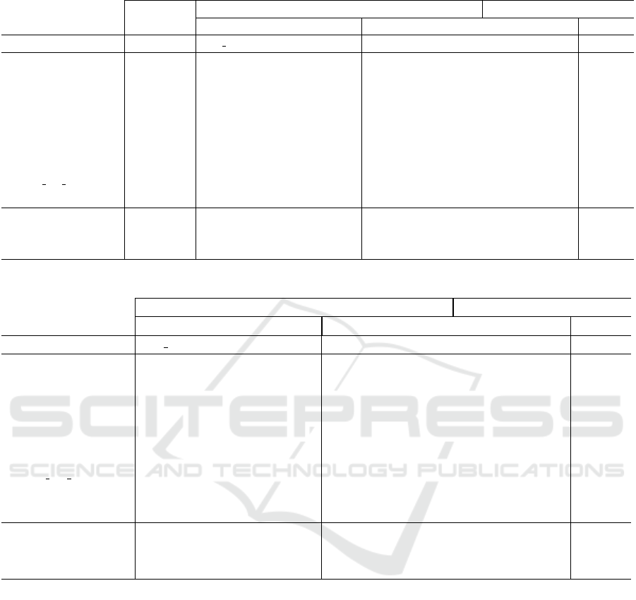
Table 5: Mean subset size for the eight feature selection methods.
Without
selection
Feature clustering-based approaches Regular approaches
Wrappers Filter Hybrid
Database # Features AP SFS FCR
NN
RCE Proposed FCR
MI
SFS CFS mRmR
Ionosphere 34 32.40 30.00 4.80 3.80 30.00 3.80 18.20 22.20
Spamdata 57 44.60 50.00 23.80 23.00 50.00 27.60 44.50 48.60
Coil-2000 85 48.20 50.00 41.20 22.00 50.00 31.80 50.00 62.50
Arrhythmia 279 166.80 50.00 20.50 26.80 50.00 42.00 27.40 40.20
Medical 1493 382.00 50.00 85.40 28.20 50.00 25.80 38.50 33.50
WarpAR10P 2400 1134.50 50.00 35.80 26.20 50.00 28.00 44.40 24.80
KTH-TIPSB 1155 298.00 50.00 30.20 15.20 50.00 50.00 42.00 21.50
Outex TC 00013 1155 266.00 50.00 75.20 21.40 50.00 50.00 8.50 50.00
NewBarktex 1155 213.60 50.00 42.60 30.60 50.00 49.80 44.40 80.80
Average (Numerical) 724.66 301.42 46.66 78.20 21.66 46.66 26.50 37.16 38.63
Average (Texture) 1155 259.20 50.00 78.20 22.40 50.00 49.80 31.63 50.77
Average 1109.62 280.31 48.33 45.50 22.03 48.33 38.15 34.40 44.70
Table 6: Average running time (in seconds) with the four feature selection methods.
Feature clustering-based Regular approaches
Wrappers Filter Hybrid
Database AP SFS FCR
NN
RCE Proposed FCR
MI
SFS CFS mRmR
ionosphere 5.21 5.32 8.35 1.17 5.82 0.34 3.41 0.08
Spamdata 15.18 22.35 2.08 63.85 21.75 4.85 15.18 0.27
Coil-2000 372.98 102.25 351.83 126.00 72.92 14.53 84.76 64.46
Arrhythmia 75.84 46.10 930.72 7.02 9.97 11.66 13.00 3.43
Medical 793.62 202.83 85.39 65.29 55.50 223.73 56.74 21.68
WarpAR10P 1535.62 335.24 340.25 15.13 93.91 58.79 38.84 16.96
Outex TC 00013 2057.7 88.88 153.25 57.16 13.42 319.81 19.76 28.70
KTH-TIPS 786.21 169.68 325.25 313.44 21.64 427.02 107.75 182.40
NewBarktex 403.15 92.24 89.53 144.00 17.94 200.09 19.95 35.81
Average (Numerical) 466.41 119.01 286.44 46.41 43.31 52.32 35.32 17.81
Average (Texture) 1082.35 116.93 143.34 171.53 17.66 315.64 49.15 82.30
Total Average 774.38 117.97 214.89 108.97 34.48 183.97 42.23 50.05
half the total computational time.
In the three image texture datasets (experiment
#2), the proposed approach comes fourth followng
FCR
MI
, CFS and mRmR respectively with a compu-
tational time of 171.53. As for the real world datasets,
the clustering time takes over 87.33 seconds which is
almost half the total computational time.
In the average over the two types of datasets, filter
approaches perform faster than wrapper ones as ex-
pected. The proposed approach comes as the fourth
method after FCR
MI
, CFS and mRmR respectively.
FCR
MI
runs faster than the other feature selection al-
gorithms due to it’s nature as a ranking filter algo-
rithm. Table 3 shows that the average time required
to find the optimal correlation threshold is 56.99 sec-
onds which is almost half of the 108.97 time required
to run the method (113.98 seconds).
On the one hand, the proposed clustering-based
sequential feature selection needs no parameter to
be adjusted to obtain a competitive accuracy but in-
creases the computation time. On the other hand, the
manual setting of the parameter could decrease this
time with no guaranty of reaching the highest accu-
racy.
5 CONCLUSION
In this paper, we have proposed a new clustering-
based sequential feature selection approach which
uses a subset search algorithm by using a filter model.
First, the algorithm removes irrelevant features, then
Clustering-based Sequential Feature Selection Approach for High Dimensional Data Classification
131

it divides the feature space into a number of clusters
with the assumption that each cluster contains corre-
lated features. Selecting one feature for each cluster
helps to select only relevant and non-redundant fea-
tures at each step of the algorithm. This approach
does not only speed up the search algorithm but also
guarantees to obtain a compact and discriminant fea-
ture space. Two experiments were conducted, the
first on six real word, numerical and ready to use
datasets and the second on three color texture im-
age databases. The obtained results were compared
to four clustering-based feature selection approaches
and three other feature selection schemes. They show
that the proposed algorithm outperforms wrapper ap-
proaches while maintaining filter ones advantages.
Compared to other filter model based approaches, our
solution provides a high level of dimensionality re-
duction, high classification accuracy with a reason-
able processing time and no parameter to be adjusted.
REFERENCES
Alimoussa, M., Vandenbroucke, N., Porebski, A., Thami,
R. O. H., Fkihi, S. E., and Hamad, D. (2019). Com-
pact color texture representation by feature selection
in multiple color spaces. In 16th International Joint
Conference on Computer Vision, Imaging and Com-
puter Graphics Theory and Applications. in Prague.
Bins, J. and Draper, B. A. (2001). Feature selection from
huge feature sets. In Proceedings Eighth IEEE Inter-
national Conference on Computer Vision. ICCV 2001,
volume 2, pages 159–165 vol.2.
Chandrashekar, G. and Sahin, F. (2014). A survey on fea-
ture selection methods. Computers & Electrical En-
gineering, 40(1):16 – 28. 40th-year commemorative
issue.
Cov
˜
oes, T. F. and Hruschka, E. R. (2011). Towards improv-
ing cluster-based feature selection with a simplified
silhouette filter. Information Sciences, 181(18):3766
– 3782.
Das, S. (2001). Filters, wrappers and a boosting-based hy-
brid for feature selection. In Proceedings of the Eigh-
teenth International Conference on Machine Learn-
ing, ICML ’01, page 74–81, San Francisco, CA, USA.
Morgan Kaufmann Publishers Inc.
Dua, D. and Graff, C. (2017). UCI machine learning repos-
itory.
Hall, M. (2000). Correlation-based feature selection for dis-
crete and numeric class machine learning. In Proceed-
ings of the 17th international conference on machine
learning (ICML-2000), pages 359–366.
Hanchuan Peng, Fuhui Long, and Ding, C. (2005). Fea-
ture selection based on mutual information crite-
ria of max-dependency, max-relevance, and min-
redundancy. IEEE Transactions on Pattern Analysis
and Machine Intelligence, 27(8):1226–1238.
Harris, D. and Niekerk, A. V. (2018). Feature clustering and
ranking for selecting stable features from high dimen-
sional remotely sensed data. International Journal of
Remote Sensing, 39(23):8934–8949.
Hsu, H.-H., Hsieh, C.-W., and Lu, M.-D. (2011). Hybrid
feature selection by combining filters and wrappers.
Expert Systems with Applications, 38(7):8144 – 8150.
Kira, K. and Rendell, L. A. (1992). The feature selection
problem: Traditional methods and a new algorithm.
In Proceedings of the Tenth National Conference on
Artificial Intelligence, AAAI’92, San Jose, California,
page 129–134.
Krier, C., Franc¸ois, D., Rossi, F., and Verleysen, M. (2007).
Feature clustering and mutual information for the se-
lection of variables in spectral data. In European Sym-
posium on Artificial Neural Networks, Computational
Intelligence and Machine Learning.
Li, B., Wang, Q., Member, J., and Hu, J. (2011). Feature
subset selection: A correlation-based SVM filter ap-
proach. IEEJ Transactions on Electrical and Elec-
tronic Engineering, 6:173 – 179.
Mitra, P., Murthy, C. A., and Pal, S. K. (2002). Unsuper-
vised feature selection using feature similarity. IEEE
Transactions on Pattern Analysis and Machine Intel-
ligence, 24(3):301–312.
Porebski, A., Vandenbroucke, N., and Hamad, D. (2015).
A fast embedded selection approach for color texture
classification using degraded LBP. In 2015 Interna-
tional Conference on Image Processing Theory, Tools
and Applications (IPTA), pages 254–259.
Porebski, A., Vandenbroucke, N., and Macaire, L. (2010).
Comparison of feature selection schemes for color
texture classification. In 2010 2nd International Con-
ference on Image Processing Theory, Tools and Appli-
cations, pages 32 – 37.
Reunanen, J. (2003). Overfitting in making comparisons
between variable selection methods. J. Mach. Learn.
Res., 3:1371–1382.
Song, Q., Ni, J., and Wang, G. (2013). A fast clustering-
based feature subset selection algorithm for high-
dimensional data. IEEE Transactions on Knowledge
and Data Engineering, 25(1):1–14.
Yousef, M., Jung, S., Showe, L., and Showe, M. (2007).
Recursive cluster elimination (rce) for classification
and feature selection from gene expression data. BMC
bioinformatics, 8:144.
Yu, L. and Liu, H. (2003). Feature selection for high-
dimensional data: A fast correlation-based filter solu-
tion. In Fawcett, T. and Mishra, N., editors, Proceed-
ings, Twentieth International Conference on Machine
Learning, pages 856–863.
Zhu, K. and Yang, J. (2013). A cluster-based sequential
feature selection algorithm. In 2013 Ninth Interna-
tional Conference on Natural Computation (ICNC),
pages 848–852.
Zhu, X., Wang, Y., Li, Y., Tan, Y., Wang, G., and Song, Q.
(2019). A new unsupervised feature selection algo-
rithm using similarity-based feature clustering. Com-
putational Intelligence, 35(1):2–22.
VISAPP 2021 - 16th International Conference on Computer Vision Theory and Applications
132