On the Link between Mesh Size Adaptation and Irregular Vertices

Daniel Zint

and Roberto Grosso

Visual Computing, Friedrich-Alexander Universit

at Erlangen-N

urnberg, Cauerstr. 11, 91058 Erlangen, Germany

Keywords:

Mesh Generation, Block-structured Grids, Irregular Vertices.

Abstract:

In numerical simulations and computer graphics meshes are often required to have varying element sizes.

High resolution, i.e. small elements, should be only used where necessary. The transition between element

sizes requires introducing irregular vertices. In this work, we examine the occurance of irregular vertices

in transition regions by setting up an advancing front triangulation that generates optimal transitions. We

establish a relation between the appearance of irregular vertices and the properties of the size function and

show that a linear transition between different element sizes can be achieved without any singularities on the

interior of the transition. Therefore, we can optimize triangulations by setting transition fronts accordingly.

These results are used to estimate properties of block-structured grids, e.g. how many blocks are required to

represent a given domain correctly.

1 INTRODUCTION

Unstructured and block-structured meshes are widely

used in computer graphics and in numerical sim-

ulations. They are favored over fully structured

meshes due to their adaptiveness to complex geom-

etry. Block-structured grids (BSGs) are on the rise

for the last decade. A BSG is a mesh where each el-

ement contains a fully structured mesh. In computer

graphics BSGs enable tensor product surface repre-

sentations, grid-based multi-resolution techniques, or

discrete pixel-based map representations (Campen,

2017). In numerical simulations, block structure

enables optimizations which reduce simulation time

drastically. For example, multigrid solvers can be

used which converge much faster than solvers that

work on unstructured meshes (Armstrong et al.,

2015).

Unstructured meshes are irreplaceable in many

applications, not just because of their adaptiveness to

complex geometry but also for their ability to adapt to

a size function. It is well known that there is a link

between changes in element size and the appearance

of irregular vertices. The more rapid the element size

changes the more irregularity is required. Neverthe-

less, at least as far as we know, this link was never in

the focus of research.

In this work, we study the appearance of irregu-

https://orcid.org/0000-0003-4491-1685

https://orcid.org/0000-0001-5965-5325

lar vertices in transition zones between different ele-

ment sizes. We describe how irregularities, element

quality, and the number of elements are connected.

We use this knowledge to achieve optimal transition

zones. These are used to remove irregular vertices

from meshes that were generated with Delaunay re-

ﬁnement or isotropic remeshing. Furthermore, we

gain a deeper understanding about BSG generation.

More precisely, we predict the properties of size-

adapted BSGs and show constraints that a size func-

tion might impose.

1.1 Singularity and Irregularity

The topology of a mesh causes singularities (Beaufort

et al., 2017). The Euler characteristic for an orientable

surface S embedded in R

χ = 2 −2g −b, (1)

where g is the genus of the surface and b the num-

ber of boundaries. Thus, for a sphere we have χ = 2,

for a disk χ = 1, and for a ring (disk with an interior

boundary) or a torus χ = 0. Theoretically, a singular-

ity corresponds to a vertex with no incident edges. In

practice a singularity is spread over several vertices.

It is more viable to talk about vertex and mesh irreg-

ularity.

Deﬁnition 1. The vertex irregularity ι

is the vertex

valence deducted with its optimal valence. For trian-

gle meshes the optimal valence for interior vertices

is 6 and for boundary vertices 4. For quad meshes

Zint, D. and Grosso, R.

On the Link between Mesh Size Adaptation and Irregular Vertices.

DOI: 10.5220/0010259200670074

In Proceedings of the 16th International Joint Conference on Computer Vision, Imaging and Computer Graphics Theory and Applications (VISIGRAPP 2021) - Volume 1: GRAPP, pages

67-74

ISBN: 978-989-758-488-6

the optimal valence for interior vertices is 4 and for

boundary vertices 3.

A vertex in a triangle mesh with valence 5 has an

irregularity of ι

= 5−6 = −1 on the interior and ι

5 −4 = 1 on the boundary. In a quad mesh a valence

5 vertex has an irregularity of ι

= 5 −4 = 1 on the

interior and ι

= 5 −3 = 2 on the boundary.

Deﬁnition 2. The mesh irregularity ι

is the sum of

all vertex irregularities,

∑

i=1

, (2)

where N is the number of vertices in the mesh and ι

is the irregularity of the vertex with index i.

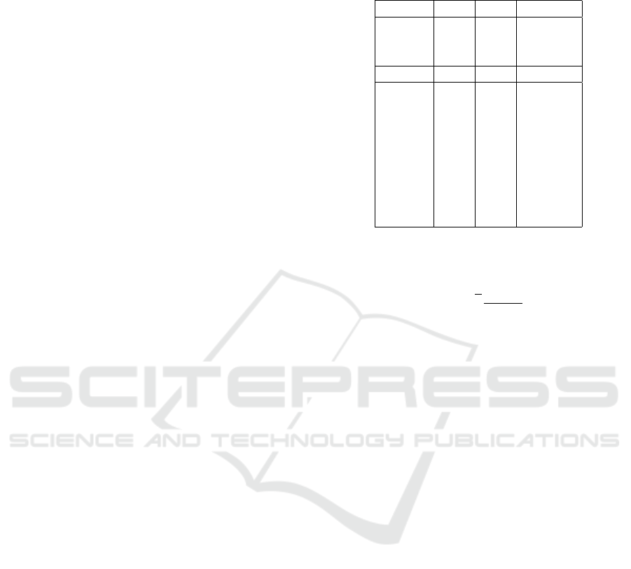
Assume the unit square is subdivided in two tri-

angles, Figure 1a. The Euler characteristic is χ = 1.

All vertices are on the boundary and thus their opti-

mal valence would be 4. Two vertices have valence 3

giving ι

= −1 and two have valence 2 which corre-

sponds to ι

= −2. Therefore, the mesh irregularity

is ι

= 2 ·(−2) + 2 ·(−1) = −6. This irregularity is

purely determined by the topology. We could reﬁne

the mesh and ﬂip edges which would create new ir-

regular vertices, but the mesh irregularity will always

remain the same as long as the genus or the number

of boundaries is not changed, see Figures 1b and 1c.

For investigating transition zones, we need more

detailed information about mesh irregularity. We dis-

tinguish between positive and negative irregularity.

Deﬁnition 3. The positive / negative mesh irregular-

ity ι

/ ι

−

is the sum of all positive / negative vertex

irregularities,

∑

i=1

(

if ι

> 0

0 otherwise,

(3)

−

∑

i=1

(

if ι

< 0

0 otherwise.

(4)

The unit square has ι

= 0 and a negative irregu-

larity of ι

−

= −6. This remains constant if we sub-

divide the mesh as all new vertices have optimal va-

lence. If edges are ﬂipped, positive and negative ir-

regularity are increased. In Figure 1c we have ι

= 1

and ι

−

= −7. Note, that both change equally as they

sum up to ι

= ι

+ ι

−

. (5)

1.2 Irregularity and Quality

Irregular vertices have a negative impact on mesh

quality. They impose an upper bound to the minimal

Table 1: Upper bound to minimal quality depending on ver-

tex valence. Quality is measured with mean ratio, minimal

angle, and ratio between longest and shortest edge.

valence q α

min

max

min

3 0.60 30 1.73

4 0.87 45 1.41

5 0.97 54 1.18

6 1.00 60 1.00

7 0.98 51 1.15

8 0.94 45 1.31

9 0.90 40 1.46

10 0.85 36 1.62

11 0.81 33 1.77

12 0.76 30 1.93

15 0.65 24 2.40

20 0.51 18 3.20

25 0.42 14 3.99

quality of their incident elements. A common way to

measure quality is using the mean ratio metric,

q = 4

√

∑

i=1

, (6)

where A is the signed area of the triangle and l

is the

length of its edges (Bank and Smith, 1997; Canann

et al., 1998; Amenta et al., 1999). We also consider

as quality measures the minimal angle, α

min

, and the

ratio between the longest and shortest edge of a tri-

angle, l

max

min

. We only measure minimal quality as

for simulations, a badly shaped element might cause

numerical instabilities. In contrast, average quality

does not contain much information and is therefore

neglected.

We compare vertex valence to the optimal mini-

mal quality of its incident triangles, Table 1. This is

an upper bound, i.e. a vertex with valence 9 might

have a quality of 0.90 but in almost any conﬁguration

it will be lower. In the optimal conﬁguration all inci-

dent edges have the same length and the same angle

between them. Usually, geometric constraints pro-

hibit this setup.

Highly irregular vertices also impose anisotropy.

A triangle with a valence four vertex has at best a quo-

tient of longest over shortest edge of 1.41. Depending

on the numerical scheme used by a simulation this

might not be acceptable.

1.3 Related Work

Adapting to a size function was considered thor-

oughly in triangle mesh generation methods. The

most common procedure is to generate a Delaunay

triangulation of a domain and then reﬁne where nec-

essary (B

ansch, 1991; Shewchuk, 1997; Cheng et al.,

GRAPP 2021 - 16th International Conference on Computer Graphics Theory and Applications

(a) Unit Square

= 2 ·(−2) + 2 ·(−1) = −6

(b) Reﬁned

= 2 ·(−2) + 2 ·(−1) + 5 ·0 = −6

= 1 ·(−2) + 5 ·(−1) + 1 ·1 = −6

Figure 1: The unit square contains four irregular vertices, two with ι

= −1 and two with ι

= −2, summing up to a mesh

irregularity of ι

= −6. Reﬁning the unit square adds ﬁve vertices with ι

= 0. An edge ﬂip affects the vertex irregularity

and therefore also the positive and negative mesh irregularity. Vertices with negative or positive irregularity are marked blue

or red correspondingly.

2012). Most of this methods add Steiner points to

the mesh and ﬂip edges to re-establish the Delau-

nay triangulation. This iterative approach, called De-

launay reﬁnement, is robust and generates unstruc-

tured meshes with high quality. Triangle is an early

software package that used the Delaunay reﬁnement

method (Shewchuk, 1996). Subsequent work focused

on improving the placement of vertices (

Ung

or, 2004;

Persson, 2005; Erten and

Ung

or, 2009; Engwirda and

Ivers, 2016).

In computer graphics, Delaunay triangulations are

generated a bit differently with isotropic remeshing

(Botsch and Kobbelt, 2004; Alliez et al., 2008). The

steps split, collapse, and smooth are performed subse-

quently to achieve almost equilateral triangles. Other

remeshing methods are based on parametrization (Al-

liez et al., 2003). Just like Delaunay reﬁnement,

remeshing methods can generate meshes with vary-

ing element sizes.

Advancing front techniques, sometimes called

paving, start at a mesh boundary and add a ring of el-

ements (Peraire et al., 1987; Blacker and Stephenson,

1991; L

ohner and Parikh, 1988). This is repeated un-

til the whole domain is ﬁlled with elements. Advanc-

ing front techniques often deliver good results along

boundaries but elements in the interior might have low

quality. Advancing front techniques regained interest

when they were combined with cross ﬁelds and are

used especially for quad mesh generation (Remacle

et al., 2013; Georgiadis et al., 2017).

None of these methods keeps track of irregular

vertices. When the research focus of meshing moved

from triangles to quads, irregularities became a topic

of bigger concern. Whereas triangles are quite ﬂex-

ible regarding irregular vertices, they are a serious

issue in quad meshes due to the lower optimal va-

lence. The introduction of cross ﬁelds was an im-

portant contribution (Klberer et al., 2007; Ray et al.,

2008; Bommes et al., 2009; Bommes et al., 2013;

Kowalski et al., 2013; Crane et al., 2010). Cross ﬁelds

are computed by solving a system of partial differen-

tial equations on the domain. Besides giving input

for advancing front techniques, cross ﬁelds also show

positions of singularities and therefore allow directly

the generation of block-structured meshes. A down-

side is that cross ﬁelds are not aware of size functions.

For mesh adaptation the grid structure needs to be re-

ﬁned by adding further singularities, e.g. Armstrong

et al. presents patterns for multiblock mesh reﬁne-

ment (Armstrong et al., 2018). Zint and Grosso try to

overcome the issue of cross ﬁelds by using a simpliﬁ-

cation method on an underlying size function to cre-

ate blocks of the correct size (Zint et al., 2019). Their

claim to representing element size correctly leads to a

large number of blocks.

2 TRIANGULATING A

TRANSITION ZONE

In this section, we study transition zones between ar-

eas of different element sizes. First, we will consider

a direct transition which does not add any further ver-

tices. Usually, the length of a transition zone is given

and the mesh generator has to ﬁnd the optimal trian-

gulation. First, we go the other way around and exam-

ine the behavior of triangulations when we adapt the

transition length. In a second step, we will add fronts

in the transition zone. Here, we go back to the orig-

inal problem and ﬁnd the optimal triangulation for a

given transition length.

The examples are generated with an advancing

front method. Therefore, we will use the term front

for the vertical lines in a mesh. For example, the unit

square consists of two fronts, one on the left and one

on the right. Furthermore, transitions are described

as patterns. The transition pattern 4:1 has 4 elements

on the ﬁrst front and 1 element on the last. If another

front with two elements is inserted in between, the

pattern is 4:2:1. The number of elements on the front

with index k is denoted by f

. Thus, the pattern with

On the Link between Mesh Size Adaptation and Irregular Vertices

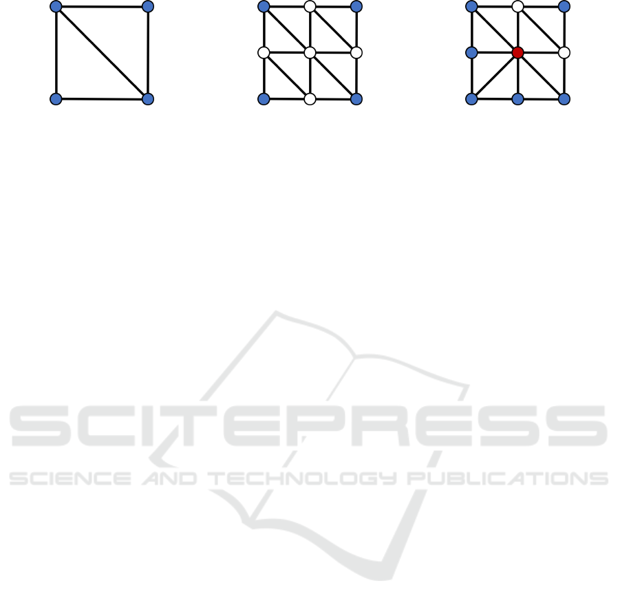
(a) 2:1 (b) 3:1 (c) 3:2

(d) 4:1 (e) 4:2 (f) 4:3

Figure 2: Delaunay triangulation on transition with only

two fronts.

four fronts is f

: f

2.1 Direct Transition

We use relative irregularity for analyzing transition.

This is advantageous as it cancels out the inﬂuence of

geometry.

Deﬁnition 4. The relative vertex irregularity

is the

vertex irregularity in comparison to the unit square as

shown in Figure 1a. This only affects the four corner

vertices.

In Figure 2a the top left vertex has

= −1 be-

cause in the unit square this vertex has three outgoing

edges and here only two. Furthermore, the vertices in

the middle and bottom left and the bottom right have

= 0. The vertex in the top right has

= +1. If f

is increased, a vertex with

= −1 is added and the

irregularity of a vertex on the right side is increased

by one, Figure 2b. The opposite happens if f

is in-

creased, Figure 2c.

Deﬁnition 5. The relative mesh irregularity

is the

sum of the relative irregularity of all vertices,

∑

i=1

. (7)

Deﬁnition 6. The relative positive / negative mesh ir-

regularity

−

is the sum of all relative positive /

negative vertex irregularities,

∑

i=1

(

> 0

0 otherwise,

(8)

−

∑

i=1

(

< 0

0 otherwise.

(9)

The cases shown in Figure 2 which only consist of

two fronts already illustrate some information about

transitions:

Figure 3: Minimal mean ratio quality of different transitions

depending on the transition-length. The domain has a height

of 1.

1. The number of elements between two fronts f

and f

k+1

( f

, f

k+1

) = f

+ f

k+1

. (10)

2. The relative positive / negative mesh irregularity

= ±( f

− f

). (11)

3. Negative irregularities are on the ﬁrst front, posi-

tive on the second. Or more general, negative ir-

regularities are on the front with more elements.

This is independent of the triangulation, as long

as triangles are not degenerated.

Additionally, we study the element quality in tran-

sition regions. We observe that triangle quality de-

creases when f

or f

increases. Triangles need to

be compressed to make room for others. The quality

of the pattern 4:3 in Figure 2f would be higher if the

transition zone would be shorter. Each transition pat-

tern has its own optimal length. The minimal element

quality of the meshes in Figure 2 when stretched in

horizontal direction is plotted in Figure 3. Some tran-

sitions always have low quality like 3:1 or 4:1. Here

arises the question if we can design such transitions

with better shaped elements by adding vertices.

2.2 Transition with Multiple Fronts

In the following, we add additional fronts in between

the left and right boundary to allow a smoother transi-

tion. Therefore, we generalize the domain descrip-

tion. A domain consists of n vertical fronts with

> f

> ... > f

. The region between fronts is trian-

gulated according to the Delaunay criterion. Further-

more, we introduce the relative irregularity of fronts.

Deﬁnition 7. The relative irregularity

f k

of a front f

is the sum of the relative irregularity of all vertices in

this front,

f k

∑

v∈f

. (12)

GRAPP 2021 - 16th International Conference on Computer Graphics Theory and Applications

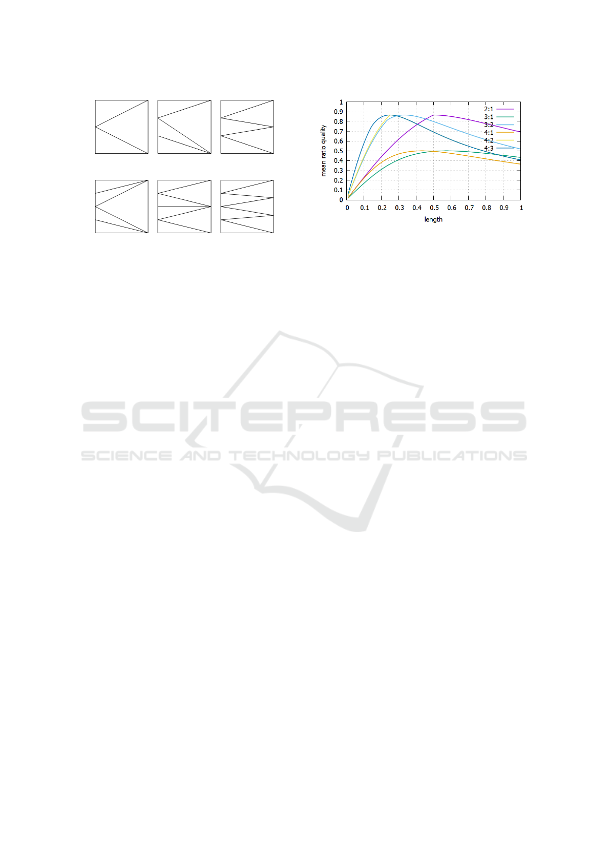
(a) 4:3:2:1 (b) 4:3:1 (c) 4:2:1

Figure 4: Transition from 4 to 1 element with different pat-

terns.

Deﬁnition 8. The relative positive / negative irregu-

larity

f k

−

f k

of a front f

is the sum of all relative

positive / negative vertex irregularities in this front,

f k

∑

v∈f

(

> 0

0 otherwise,

(13)

−

f k

∑

v∈f

(

< 0

0 otherwise.

(14)

Figure 4 shows different transitions from 4 el-

ements to 1. In Figure 4a two fronts are added.

The second front has f

= 3 elements and the third

= 2. Thus, the number of edges is decreased

by one between all fronts. The ﬁrst front (which

is the left boundary) has a relative irregularity of

f 1

= −1, the second and third front have no irregular-

ity

f 2

f 3

= 0, and the right boundary has one pos-

itive irregularity

f 4

= 1. Thus, the additional fronts

reduced the relative mesh irregularity from

= ±3

= ±1.

Inserting fronts can be seen as stacking transition

zones. In the 4:2:1 example in Figure 4c we have a

transition from 4:2 and another from 2:1. The number

of elements can be computed as

( f

, f

,..., f

) = N

( f

, f

) + N

( f

, f

) + ...

= ( f

+ f

) + ... + ( f

n−1

+ f

)

= f

+ f

+ 2

n−1

∑

i=2

. (15)

The ﬁrst transition generates 2 positive irregulari-

ties on the ﬁrst front and two negative on the sec-

ond. The second transition generates 1 positive ir-

regularity on the second front and one negative on the

third. The positive and one negative irregularity on

the second front are canceling each other out giving

f 2

= 1 −2 = −1. This generalizes to the relative ir-

regularity of a front f

f k

= f

k−1

−2 f

+ f

k+1

with 1 ≤k ≤n. (16)

This holds also for the boundary fronts when we as-

sume that element size is constant outside of the tran-

sition zone, i.e. f

= f

and f

n+1

= f

. From Equation

16 it follows that irregularities only appear when the

gradient of the size function is not constant.

Figure 5: Minimal quality of different transitions between

four and one element depending on the transition-length.

With Equation 16 and f

k−1

> f

k+1

for

1 < k < n we can compute the relative positive and

negative mesh irregularity:

f 1

= f

−2 f

+ f

= −f

+ f

< 0 (17)

f n

= f

n−1

−2 f

+ f

n+1

= f

n−1

− f

> 0 (18)

f k

≥ 0 if f

k−1

+ f

k+1

≤ 2 f

(19)

∑

k=1

(

f k

> 0

0 otherwise.

(20)

−

∑

k=1

(

f k

< 0

0 otherwise.

(21)

∑

k=2

f k

if f

k−1

+ f

k+1

≤ 2 f

(22)

−

= f

− f

if f

k−1

+ f

k+1

≤ 2 f

(23)

Equations 19, 22, and 23 are of special interest as they

give hints about optimal transition zones. For the case

k−1

+ f

k+1

= 2 f

we can avoid irregularities within

the transition zone completely. Thus, the descent in

edge size should be equal between all fronts which

corresponds to a linear size function. Non-linear size

functions will always impose irregularities. Figure 4a

shows an optimal transition. Figure 4b and 4c have

the same relative mesh irregularity.

In terms of quality, it might not always be the best

choice to opt for the lowest possible amount of irregu-

lar vertices. Figure 5 shows the minimal quality of the

meshes from Figure 4 when stretched along the hori-

zontal axis. The 4:3:2:1 pattern is preferable when the

transition is longer. If the transition should be more

rapid, the 4:2:1 mesh is the better choice. Thus, de-

pending on the gradient size of a size function one

might choose a different pattern. In any case, asym-

metric transitions like 3:1 should be avoided as they

impose low quality while having the same relative ir-

regularity as symmetric patterns.

On the Link between Mesh Size Adaptation and Irregular Vertices

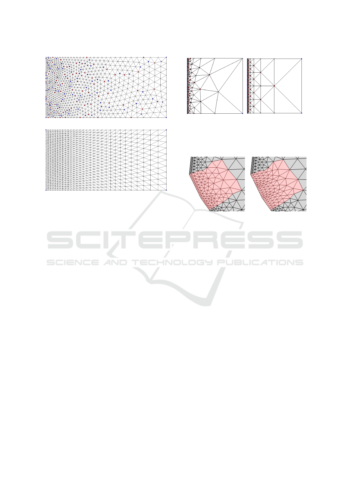
(a) remeshing

(b) optimal

Figure 6: Transition from 40 to 10 elements once achieved

with remeshing, once by computing the optimal transition.

Negative irregularities are marked blue, positive irregulari-

ties are red.

3 COMPARISON TO ADAPTIVE

REMESHING

A simple way to apply a size function to a mesh is by

using adaptive remeshing like the one of Botsch and

Kobbelt (Botsch and Kobbelt, 2004). Even though

remeshing delivers overall good quality, it also gen-

erates many unnecessary irregular vertices. In Fig-

ure 6a we apply the remeshing of Botsch and Kobbelt

to a transition from 40 to 10 elements, assuming a

linear size function. The average triangle quality is

0.98 but the minimal quality only 0.39. By computing

the optimal transition we only get irregularities on the

left and right boundary and achieve a minimal qual-

ity of 0.79. The average quality is 0.86. Both meshes

have almost the same number of elements, remesh-

ing produces 1512 and the optimal contains 1 500 el-

ements. In Figure 7, we applied a size function which

decreases exponentially. Similar issues are observed

here. Remeshing only achieved a minimal quality of

0.33 and an average quality of 0.75 whereas the op-

timal transition has a minimal and average quality of

0.87. Remeshing generates 313 triangles, the optimal

transition has 381.

Also Delaunay reﬁnement can be improved by

identifying transition zones and exchanging them

with the optimal transition. In Figure 8 we selected

(a) remeshing (b) optimal

Figure 7: Transition from 128 to 1 element with an expo-

nential size function once achieved with remeshing, once

by computing the optimal transition. Negative irregularities

are marked blue, positive irregularities are red.

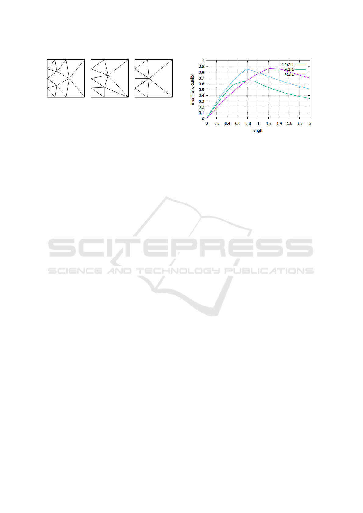
(a) Delaunay triangulation (b) optimal

Figure 8: Remeshing a rectangular region in a mesh gener-

ated with Delaunay reﬁnement reduces the irregularity sig-

niﬁcantly.

a rectangular region of a mesh designed for ﬂuid

simulations. Deploying optimal transition reduces

the amount of irregular vertices signiﬁcantly from 63

down to 8. The minimal quality of this region de-

creases slightly from 0.76 to 0.75. This value could

be further improved by smoothing the boundaries of

the rectangular region. The number of elements goes

down from 205 to 189.

4 PROPERTY-ESTIMATION OF

BLOCK-STRUCTURED GRIDS

Optimal transitions can be used to estimate proper-

ties of BSGs. Assume, the marked region in Figure 9

should be subdivided into triangular blocks. The re-

gion is a transition from 28 to 4 with 10 or 11 fronts.

This can be approximated by a relation of 7:1 and one

or two interior fronts. Thus, the optimal pattern would

be either 7:5:3:1 or 7:4:1, Figure 10. Reﬁning these

patterns two times with uniform subdivision results in

BSGs with 16 triangles per block that are comparable

to the unstructured mesh, Table 2.

The size function imposes that the region should

consist of at least 16 blocks. The minimal number

of blocks for a 7:1 transition would be 8, but besides

GRAPP 2021 - 16th International Conference on Computer Graphics Theory and Applications

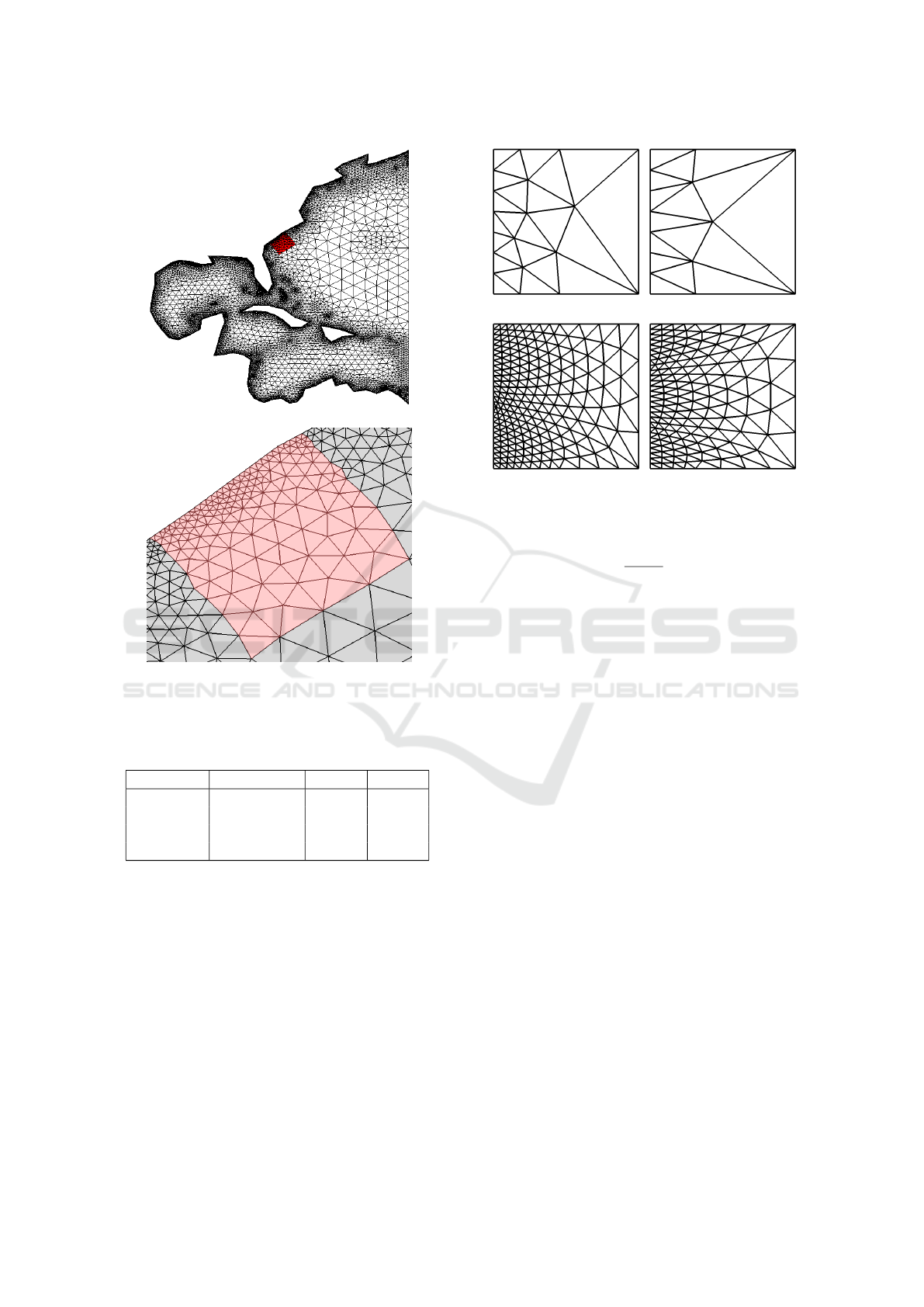
Figure 9: A rectangular transition region within an unstruc-

tured triangle mesh. The transition gives information about

the number of blocks that is required to represent the do-

main correctly.

Table 2: BSG property estimation.

unstructured 7:5:3:1 7:4:1

# blocks 24 16

# triangles 297 384 256

min

0.75 < 0.98 < 0.90

40 2 3

generating large irregularities, this would also lead to

anisotropy and is therefore not advisable. Also a 7:2:1

pattern would be possible which would then result in

14 blocks but already 16 blocks have less triangles

than in the unstructured case. Reducing the number

of blocks only makes sense if we can reﬁne the blocks

further. This is constrained by the coarsest bound-

ary which only contains four elements. Considering a

larger region does not solve this issue as the relation

between ﬁne to coarse will remain 7:1.

If 16 triangles build one block, we can compute

the number of blocks that is required for representing

all 18578 triangles of the unstructured mesh,

(a) 7:5:3:1 (b) 7:4:1

Figure 10: Transition from 7 to 1 element either with one or

two additional fronts.

block

18578

≈ 1161. (24)

This is just a rough estimation but it hints at the

minimal amount of blocks. It will not be possible

to represent this domain with 10, 100, or even 500

blocks if element size and quality should be pre-

served.

Depending on the simulation the size function

might only be a lower limit, i.e. elements might be

smaller but not larger than the value given by the size

function. In that case, much less blocks can be gener-

ated as the relation between ﬁne and coarse can be set

to 4:1 or even 2:1 and blocks may contain more ele-

ments than just 16. To enable this transition the num-

ber of elements needs to be increased. If one fourth

of the triangles would be reﬁned uniformly we would

get around 32510 triangles. Assuming that one block

would consist of 64 triangles, the mesh could be rep-

resented by approximately 510 blocks.

In general, the size function gradient determines

the required number of blocks. The larger the gradi-

ent the more blocks are required. This issue can not

be solved by smoothing as this only adapts the mesh

locally.

5 CONCLUSIONS

We studied the transition between different element

sizes in triangular meshes. We demonstrated that the

minimum number of irregularities in a transition zone

can be computed with a simple formula and studied

On the Link between Mesh Size Adaptation and Irregular Vertices

the inﬂuence of irregularities on mesh quality. We

also show that a transition requires no interior singu-

larities if the size function gradient is constant. With

this knowledge, we can remove irregularities from

meshes generated by remeshing or with Delaunay

reﬁnement without decreasing quality signiﬁcantly.

Furthermore, we present a technique to estimate the

required number of blocks for correctly representing

a domain while satisfying the constraints imposed by

a size function. In the future, we plan to extend this

concepts to more complex problems.

REFERENCES

Alliez, P., De Verdiere, E. C., Devillers, O., and Isenburg,

M. (2003). Isotropic surface remeshing. In 2003

Shape Modeling International., pages 49–58. IEEE.

Alliez, P., Ucelli, G., Gotsman, C., and Attene, M. (2008).

Recent advances in remeshing of surfaces. In Shape

analysis and structuring, pages 53–82. Springer.

Amenta, N., Bern, M., and Eppstein, D. (1999). Optimal

point placement for mesh smoothing. Journal of Al-

gorithms, 30(2):302–322.

Armstrong, C. G., Fogg, H. J., Tierney, C. M., and Robin-

son, T. T. (2015). Common themes in multi-block

structured quad/hex mesh generation. Procedia En-

gineering, 124:70 – 82. 24th International Meshing

Roundtable.

Armstrong, C. G., Li, T. S., Tierney, C., and Robinson, T. T.

(2018). Multiblock mesh reﬁnement by adding mesh

singularities. In International Meshing Roundtable,

pages 189–207. Springer.

Bank, R. E. and Smith, R. K. (1997). Mesh smoothing using

a posteriori error estimates. SIAM Journal on Numer-

ical Analysis, 34(3):979–997.

ansch, E. (1991). Local mesh reﬁnement in 2 and 3 di-

mensions. IMPACT of Computing in Science and En-

gineering, 3(3):181–191.

Beaufort, P.-A., Lambrechts, J., Henrotte, F., Geuzaine, C.,

and Remacle, J.-F. (2017). Computing cross ﬁelds

a pde approach based on the ginzburg-landau theory.

Procedia engineering, 203:219–231.

Blacker, T. D. and Stephenson, M. B. (1991). Paving: A

new approach to automated quadrilateral mesh gener-

ation. International Journal for Numerical Methods

in Engineering, 32(4):811–847.

Bommes, D., Lvy, B., Pietroni, N., Puppo, E., Silva, C.,

Tarini, M., and Zorin, D. (2013). Quad-mesh gener-

ation and processing: A survey. Computer Graphics

Forum, 32(6):51–76.

Bommes, D., Zimmer, H., and Kobbelt, L. (2009). Mixed-

integer quadrangulation. ACM Trans. Graph., 28(3).

Botsch, M. and Kobbelt, L. (2004). A remeshing approach

to multiresolution modeling. In Proceedings of the

2004 Eurographics/ACM SIGGRAPH symposium on

Geometry processing, pages 185–192.

Campen, M. (2017). Partitioning surfaces into quadrilat-

eral patches: A survey. Computer Graphics Forum,

36(8):567–588.

Canann, S. A., Tristano, J. R., Staten, M. L., et al. (1998).

An approach to combined laplacian and optimization-

based smoothing for triangular, quadrilateral, and

quad-dominant meshes. In IMR, pages 479–494. Cite-

seer.

Cheng, S.-W., Dey, T. K., and Shewchuk, J. (2012). Delau-

nay mesh generation. CRC Press.

Crane, K., Desbrun, M., and Schr

oder, P. (2010). Trivial

connections on discrete surfaces. In Computer Graph-

ics Forum, volume 29, pages 1525–1533. Wiley On-

line Library.

Engwirda, D. and Ivers, D. (2016). Off-centre steiner

points for delaunay-reﬁnement on curved surfaces.

Computer-Aided Design, 72:157–171.

Erten, H. and

Ung

or, A. (2009). Quality triangulations with

locally optimal steiner points. SIAM Journal on Sci-

entiﬁc Computing, 31(3):2103–2130.

Georgiadis, C., Beaufort, P., Lambrechts, J., and Remacle,

J. (2017). High quality mesh generation using cross

and asterisk ﬁelds: Application on coastal domains.

CoRR, abs/1706.02236.

Klberer, F., Nieser, M., and Polthier, K. (2007). Quadcover

- surface parameterization using branched coverings.

Computer Graphics Forum, 26(3):375–384.

Kowalski, N., Ledoux, F., and Frey, P. (2013). A pde based

approach to multidomain partitioning and quadrilat-

eral meshing. In Proceedings of the 21st international

meshing roundtable, pages 137–154. Springer.

ohner, R. and Parikh, P. (1988). Generation of three-

dimensional unstructured grids by the advancing-front

method. International Journal for Numerical Methods

in Fluids, 8(10):1135–1149.

Peraire, J., Vahdati, M., Morgan, K., and Zienkiewicz,

O. C. (1987). Adaptive remeshing for compressible

ﬂow computations. Journal of computational physics,

72(2):449–466.

Persson, P.-O. (2005). Mesh generation for implicit geome-

tries. PhD thesis, Massachusetts Institute of Technol-

ogy.

Ray, N., Vallet, B., Li, W. C., and L

evy, B. (2008). N-

symmetry direction ﬁeld design. ACM Transactions

on Graphics (TOG), 27(2):1–13.

Remacle, J. F., Henrotte, F., Baudouin, T. C., Geuzaine, C.,

echet, E., Mouton, T., and Marchandise, E. (2013).

A frontal delaunay quad mesh generator using the L ∞

norm. International Journal for Numerical Methods

in Engineering, 94(5):494–512.

Shewchuk, J. R. (1996). Triangle: Engineering a 2d quality

mesh generator and delaunay triangulator. In Work-

shop on Applied Computational Geometry, pages

203–222. Springer.

Shewchuk, J. R. (1997). Delaunay reﬁnement mesh gener-

ation. Technical report, Carnegie-Mellon Univ Pitts-

burgh Pa School of Computer Science.

Ung

or, A. (2004). Off-centers: A new type of steiner points

for computing size-optimal quality-guaranteed delau-

nay triangulations. In Latin American Symposium on

Theoretical Informatics, pages 152–161. Springer.

Zint, D., Grosso, R., Aizinger, V., and K

ostler, H. (2019).

Generation of block structured grids on complex

domains for high performance simulation. Com-

putational Mathematics and Mathematical Physics,

59(12):2108–2123.

GRAPP 2021 - 16th International Conference on Computer Graphics Theory and Applications