Explaining Inaccurate Predictions of Models through

k-Nearest Neighbors

Zeki Bilgin

1 a

and Murat Gunestas

2 b

Arcelik Research, Istanbul, Turkey

Cyphore Cyber Security and Forensics Initiative, Istanbul, Turkey

Keywords:

XAI, Explainable AI, Deep Learning, Nearest Neighbors, Neural Networks.

Abstract:

Deep Learning (DL) models exhibit dramatic success in a wide variety of ﬁelds such as human-machine

interaction, computer vision, speech recognition, etc. Yet, the widespread deployment of these models partly

depends on earning trust in them. Understanding how DL models reach a decision can help to build trust

on these systems. In this study, we present a method for explaining inaccurate predictions of DL models

through post-hoc analysis of k-nearest neighbours. More speciﬁcally, we extract k-nearest neighbours from

training samples for a given mispredicted test instance, and then feed them into the model as input to observe

the model’s response which is used for post-hoc analysis in comparison with the original mispredicted test

sample. We apply our method on two different datasets, i.e. IRIS and CIFAR10, to show its feasibility on

concrete examples.

1 INTRODUCTION

Explainable Artiﬁcial Intelligence (XAI) is an emerg-

ing and popular research topic in AI community,

which aims to understand and explain underlying

decision-making mechanism of AI-based systems

(Arrieta et al., 2020). Being able to explain how AI

systems reach a decision in an understandable way for

human beings is crucial to build trust on these sys-

tems (Barbado and Corcho, 2019; Chakraborti et al.,

2020; Ribeiro et al., 2016). This is particularly im-

portant for some use cases such as autonomous ve-

hicles, security, ﬁnance, defense, and medical diag-

nosis, where an inaccurate decision could cause non-

recoverable damages (Arrieta et al., 2020; Tjoa and

Guan, 2019; Holzinger et al., 2019). Due to the im-

portance of the issue, DARPA decided to launch an

XAI program in May 2017, with the objective of cre-

ating AI systems whose learned models and decisions

can be understood and appropriately trusted by end

users (Gunning and Aha, 2019). The need for an ex-

planation of an algorithmic decision that signiﬁcantly

affects human beings is also mentioned in European

Union regulations (Goodman and Flaxman, 2017).

The problem actually arises from the black-box

https://orcid.org/0000-0002-8613-4071

https://orcid.org/0000-0001-8096-689X

characteristics displayed by advanced AI models.

Particularly, the rise of neural network-based Deep

Learning (DL) models that exhibit dramatic success

in a wide range of tasks from load forecasting (Us-

tundag Soykan et al., 2019) to vulnerability prediction

(Bilgin et al., 2020), by relying on efﬁcient learning

algorithms with huge parametric space, makes them

be considered as complex black-box models (Arri-

eta et al., 2020; Castelvecchi, 2016). Therefore, to

be considered practical, a model’s decision-making

mechanism either needs to be more transparent, or

provides hints on what could perturb the model (Hall,

2018). In this study, we focus on this issue and seek

to understand why a model makes inaccurate pre-

dictions by performing experimental analysis on two

different datasets from two different domains. The

ﬁrst dataset we consider is IRIS dataset (Dua and

Graff, 2017), which consists of 50 samples from each

of three species of Iris, and the second one is CI-

FAR10 (Krizhevsky et al., 2009), which consists of

60000 32x32 colour images in 10 different classes,

with 6000 images per class. Our approach is a kind

of post-hoc analysis of mispredictions based on k-

nearest neighbours of training samples corresponding

to inaccurately predicted test instance. Our motiva-

tion for focusing on inaccurate predictions is that ex-

plaining a model’s mispredictions may be more criti-

cal with respect to accurate predictions in some situa-

228

Bilgin, Z. and Gunestas, M.

Explaining Inaccurate Predictions of Models through k-Nearest Neighbors.

DOI: 10.5220/0010257902280236

In Proceedings of the 13th International Conference on Agents and Artiﬁcial Intelligence (ICAART 2021) - Volume 2, pages 228-236

ISBN: 978-989-758-484-8

tions that require responsibility.

In our proposed method, when a model makes a

misprediction for a certain test input, we ﬁrst extract

k-nearest neigbours from the training set based on a

speciﬁc distance calculation approach, and then feed

these extracted samples into the model as input to get

auxiliary predictions which will be used for post-hoc

analysis. Considering the original misprediction to-

gether with auxiliary predictions, we perform both

sample-based individual analyses and collective sta-

tistical analysis on them. The main contribution of

this study is that it provides a methodology, with

supportive experimental results, based on the analy-

sis of the model’s behaviour on k-nearest neighbors

of the mispredicted sample to understand the reasons

for the model’s inaccurate estimations, by presenting

more appropriate distance calculation method in near-

est neighbour search when dealing with image data.

The rest of the paper is organized as follows: First,

in Section 2, we give an overview of related work

and explain how our work differs from prior studies.

Then, in Section 3, we present our post-hoc analysis

method to explain inaccurate decisions of deep learn-

ing models. Section 4 includes our experimental anal-

ysis for two different datasets. Finally, we conclude

our work by giving ﬁnal remarks.

2 RELATED WORK

There are certain concepts that are highly related with

model explainability, and some studies provide well-

deﬁned meanings of these concepts and discuss their

differences. For example, in (Roscher et al., 2020),

the authors review XAI in view of applications in the

natural sciences and discuss three main relevant el-

ements: transparency, interpretability, and explain-

ability. Transparency can be considered as the oppo-

site of the “black-boxness” (Lipton, 2018), whereas

interpretability pertains to the capability of making

sense of an obtained ML model (Roscher et al., 2020).

The work (Holzinger et al., 2019) introduces the no-

tion of causability as a property of a person in contrast

to explainability which is a property of a system, and

discusses their difference for medical applications.

Some other studies providing comprehensive outline

of the different aspects of XAI are (Chakraborti et al.,

2020), (Arrieta et al., 2020) and (Cui et al., 2019).

Rule Extraction. One common and longstand-

ing approach used to explain AI decisions is the rule

extraction, which aims to construct a simpler coun-

terpart of a complex model via approximation such

as building a decision tree or linear model leading

to similar predictions of the complex model. An

early work in this category belongs to Ribeiro et

al. (Ribeiro et al., 2016), who present a method

to explain the predictions of any model by learning

an interpretable sparse linear model in a local re-

gion around the prediction. In another work (Bar-

bado and Corcho, 2019), the authors evaluate some

of the most important rule extraction techniques over

the OneClass SVM model which is a method for

unsupervised anomaly detection. In addition, they

propose algorithms to compute metrics related with

XAI regarding the “comprehensivility”, “representa-

tiveness”, “stability” and “diversity” of the rules ex-

tracted. The works (Bologna and Hayashi, 2017;

Bologna, 2019; Bologna and Fossati, 2020) present

a few different variants of a similar propositional

rule extraction technique from several neural network

models trained for various tasks such as sentiment

analysis, image classiﬁcation, etc.

Post-hoc Analysis. Another widely adopted ap-

proach is the post-hoc analysis, which involves dif-

ferent techniques trying to explain the predictions of

ML models that are not transparent by design. In

this category, the authors of (Petkovic et al., 2018)

develop frameworks for post-training analysis of a

trained random forest with the objective of explaining

the model’s behavior. Adopting a user-centered ap-

proach, they generate an easy to interpret one page ex-

plainability summary report from the trained RF clas-

siﬁer, and claim that the reports dramatically boosted

the user’s understanding of the model and trust in the

system. In another study (Hendricks et al., 2016),

the authors bring a visual explanation method that fo-

cuses on the discriminating properties of the visible

object, jointly predicts a class label, and explains why

the predicted label is appropriate for the image.

A model explanation technique relevant to our

proposed method is the explanation by example as a

subcategory of the post-hoc analysis approach (Arri-

eta et al., 2020). As an early work in this category,

Bien et al. (Bien and Tibshirani, 2011) develop a Pro-

totype Selection (PS) method, where a prototype can

be considered as a very close or identical observation

in the training set, that seeks a minimal representa-

tive subset of samples with the objective of making

the dataset more easily “human-readable”. Aligned

with (Bien and Tibshirani, 2011), Li et al. (Li et al.,

2018) use prototypes to design an interpretable neural

network architecture whose predictions are based on

the similarity of the input to a small set of prototypes.

Similarly, Caruena et al. (Caruana et al., 1999) sug-

gest that a comparison of the representation predicted

by a single layer neural network with the represen-

tations learned on its training data would help iden-

tify points in the training data that best explain the

Explaining Inaccurate Predictions of Models through k-Nearest Neighbors

229

prediction made. The work (Papernot and McDaniel,

2018) exhibits a particular example of classical ML

model enhanced with its DL counterpart (Deep Near-

est Neighbors DkNN), where the neighbors consti-

tute human-interpretable explanations of predictions

including model failures. Our own study differs from

these studies in that (i) we focus on diagnosing pos-

sible root causes of a model’s inaccurate predictions

and thus try to explain what perturbs the model, (ii)

we do not design a new neural network structure (e.g.

on contrary to (Li et al., 2018)), (iii) we perform

post-hoc analyses based on the model’s extra predic-

tions when the k-nearest neighbors of training sam-

ples of the mispredicted test inputs are entered into

the model, and (iv) we ﬁnd k-nearest neighbors based

on the distance calculated according to the features

extracted at internal layer of convolutional neural net-

work (CNN) used.

3 EXPLAINING INACCURATE

PREDICTIONS VIA k-NEAREST

NEIGHBORS

Our objective is to understand why a model makes in-

accurate prediction on a certain test sample. If this

goal is achieved, the model can be improved by tak-

ing appropriate actions based on revealed root causes

of the inaccurate predictions. To this end, we present

a post-hoc analysis method based on analysis of the

model’s prediction response on k-nearest neighbors of

the training samples corresponding to the test sample

in question. To put it another way, we ﬁrst extract

the k-nearest neighbors from the training dataset for

a given mispredicted test input, and then feed these

extracted k-nearest neighbors into the same model

and get the auxiliary predictions for these extracted k-

nearest neighbors. Then, we perform post-hoc analy-

ses on these additional predictions together with orig-

inal inaccurate test prediction by seeking to reveal

what could perturb the model. Figure 1 depicts high-

level schema of our methodology.

As depicted in Figure 1, our method relies on ex-

tracting k-nearest neighbors from training dataset for

a given test input, and therefore, it is highly crucial

for our method how to calculate distance between two

samples, which forms the basis of the nearness crite-

rion between the two samples. In the following sub-

section, we discuss this issue in detail from the per-

spective of two different datasets in two different do-

mains.

Table 1: Sample instances from IRIS dataset.

Flower Attributes

Name sepal

length

(cm)

sepal

width

(cm)

petal

length

(cm)

petal

width

(cm)

Setosa 5.1 3.5 1.4 0.2

Setosa 4.9 3.0 1.4 0.2

Versicolor 7.0 3.2 4.7 1.4

Versicolor 5.5 2.3 4.0 1.3

Virginica 6.3 3.3 6.0 2.5

Virginica 5.8 2.7 5.1 1.9

Table 2: 3-nearest neighbours of a sample based on eu-

clidean distance in IRIS dataset.

Flower Attributes Nearest

Neighbors

Name sepal

length

(cm)

sepal

width

(cm)

petal

length

(cm)

petal

width

(cm)

euclidean

distance

(cm)

Setosa 5.1 3.5 1.4 0.2 -

Setosa 5.1 3.5 1.4 0.3 0.100

Setosa 5.0 3.6 1.4 0.2 0.141

Setosa 5.1 3.4 1.5 0.2 0.141

3.1 Extracting k-Nearest Neighbors

There are many alternative metrics that can be used

to measure distance between two samples. For exam-

ple, one of the most widely used metric is euclidean

distance, which calculates element-wise distance be-

tween corresponding elements of two item to be com-

pared as formulated in Equation 1.

L(x, y) =

∑

i=1

− y

)

(1)

where x and y are a pair of samples in an n-

dimensional feature space.

Euclidean distance can be safely used to measure

distance between two samples especially when these

samples are constituted of features with numeric val-

ues. For example, in IRIS dataset, each instance is

represented with four features as indicated in Table 1.

These are sepal length, sepal width, petal length, and

petal width in cm of the iris ﬂower. The euclidean-

based 3-nearest neighbours of the ﬁrst instance in Ta-

ble 1 are given in Table 2. For this particular case,

it is easy to observe the similarity between the given

instance and its nearest neighbours as there are small

deviations on some of the feature values.

However, when we deal with an image dataset

such as CIFAR10, calculating euclidean distance di-

rectly between two images may not be appropriate to

ICAART 2021 - 13th International Conference on Agents and Artiﬁcial Intelligence

230

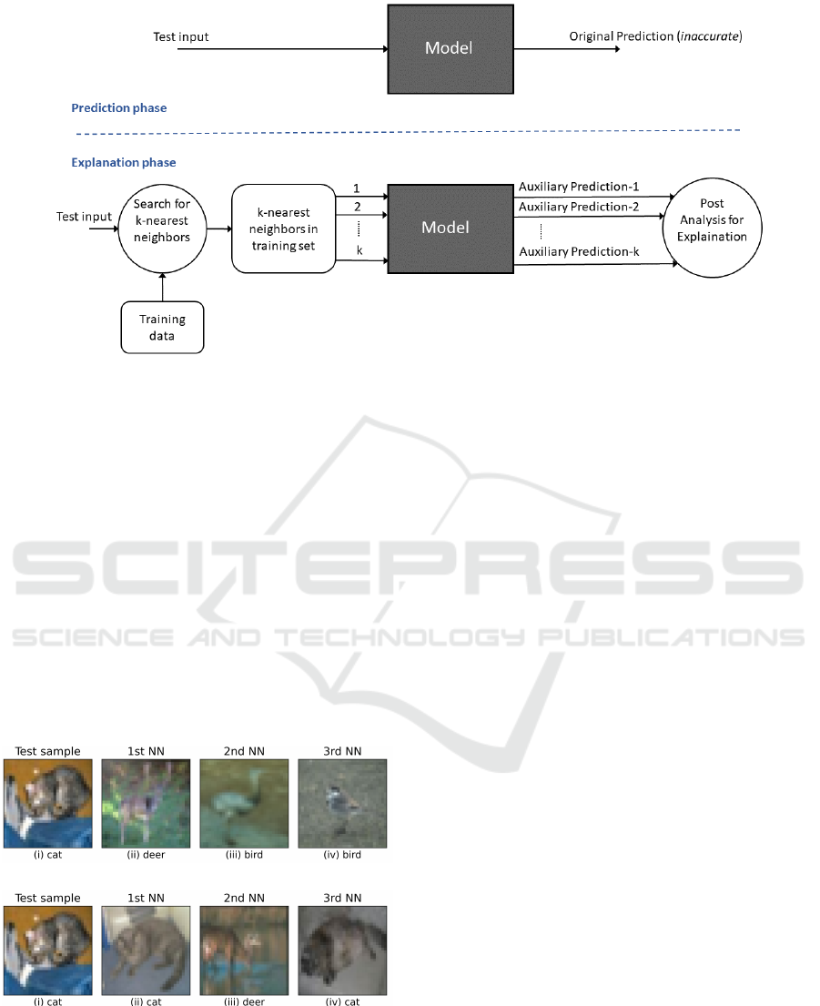
Figure 1: Overview of the method.

ﬁnd nearest neighbours. This is because the similar-

ity between two images is something complicated and

requires sophisticated analysis. For example, con-

sider two images consisting of the same object but

in different locality in the images (e.g. the object is

located in top-left of the ﬁrst image, whereas it is

in the bottom-right of the second image). In such a

case, the euclidean distance between these two im-

ages could be a large number, implying that these two

images have not any common property, although the

opposite is the case. To illustrate this, as an example,

we found 3-nearest neighbours of an image from CI-

FAR10 dataset based on euclidean distance between

images, and demonstrate them in Figure 2a.

As seen in Figure 2a, the 3-nearest neighbours

(a)

(b)

Figure 2: The 3-nearest neighbours of the training set for the

very ﬁrst sample of the test set in CIFAR10 dataset based

on (a) euclidean distance directly between images and (b)

euclidean distance on the extracted features at the internal

layers of the neural network.

of the given test sample (index=0 in the original CI-

FAR10 test dataset) are images of deer, bird, and bird

respectively, which validates our claim that similarity

between images is a bit more complicated than simi-

larity between vectoral data. Therefore, while ﬁnding

nearest neighbours in CIFAR10 dataset, instead of di-

rectly applying euclidean distance calculation on im-

ages, we ﬁrst get the extracted image features at inter-

nal layers of the utilized convolutional neural network

as depicted in Figure 3, and then calculate euclidean

distance on these features which is in the form of a

vector consisting of numeric data. We hypothesise

that this approach could give more meaningful and

appropriate nearest neighbours. To validate this, for

the same test sample given in Figure 2a, we found the

3-nearest neighbours based on the euclidean distance

between the extracted features at the internal layers

of the neural network as demonstrated in Figure 2b.

As seen in Figure 2b, the 1

and 3

nearest neigh-

bours are images of a cat, which really look like the

test sample, and the 2

nearest neighbour is an image

of deer, which is also meaningful as it has observable

similar patterns (e.g. curves) with the test sample. As

a result, when dealing with CIFAR10 dataset, we ﬁnd

nearest neighbours based on euclidean distance be-

tween the extracted features at internal layers of the

neural network to be used.

3.2 Post-hoc Analysis

When we encounter an incorrect prediction of the

model, we ﬁrst extract the k-nearest neighbours in

the training set based on the incorrectly predicted test

sample as described in the previous part, and then give

them as input to the model in order to obtain auxiliary

Explaining Inaccurate Predictions of Models through k-Nearest Neighbors

231

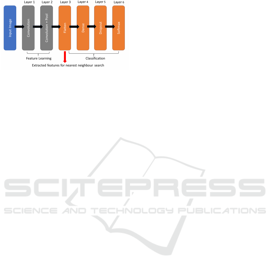
Figure 3: Getting the features extracted at the internal layers

of CNN, which is used for distance calculations in k-nearest

neighbor search.

predictions. In the post-hoc analyses, we compare the

original inaccurate prediction with the auxiliary pre-

dictions with the objective of revealing possible cause

of the misprediction in question. There may appear

different cases as explained below:

• Case-I: A sample of k-nearest neighbour is

belong to same category with the correspond-

ing inaccurately predicted test sample, and the

model makes accurate prediction when this near-

est neighbour is given the model as input. This

situation is a sign that the model actually ﬁts well

and inaccurate prediction of the test sample is an

unexpected circumstance.

• Case-II: A sample of k-nearest neighbour is be-

long to same category with the corresponding in-

accurately predicted test sample, but the model

makes inaccurate prediction when this nearest

neighbour is given the model as input. This sit-

uation implies that the model may not be ﬁtted

very well which could also be the root cause of

the original misprediction of the test sample.

• Case-III: A sample of k-nearest neighbour is

belong to different category with respect to the

corresponding inaccurately predicted test sample,

and the model makes accurate prediction when

this nearest neighbour is given the model as in-

put. This situation can imply that this nearest

neighbour may have some disruptive effect on the

model’s prediction performance on the test sam-

ple in question, because the fact that the model

makes accurate prediction on a nearest neighbour

in different category means that the model learnt

to yield this nearest neighbour’s category when

identical inputs are given, which would be an in-

accurate prediction for the corresponding test in-

put. On the other hand, if the majority of the near-

est neighbours falls in this case, then the mispre-

dicted test instance is likely to be an outlier or lo-

cated near the boundaries of data points.

• Case-IV: A sample of k-nearest neighbour is be-

long to different category with respect to the

corresponding inaccurately predicted test sam-

ple, and the model makes inaccurate prediction

when this nearest neighbour is given the model

as input. How this situation affects the model’s

behaviour on the related test sample partly de-

pends on whether this misprediction of the near-

est neighbour is the same with the original inac-

curate test prediction or not. For Case IV, suppose

the model’s prediction for the nearest neighbour is

different than the original test misprediction. This

situation does not give any clue about the model’s

inaccurate prediction for the test sample.

• Case-V: A sample of k-nearest neighbour is be-

long to different category with respect to the

corresponding inaccurately predicted test sample,

and the model makes inaccurate prediction when

this nearest neighbour is given the model as input.

Moreover, this misprediction is the same with the

original test misprediction. Such a situation im-

plies that the model behaves in harmony with the

nearest neighbours, and may also point that the

test sample is outlier of its own category.

4 EXPERIMENTAL ANALYSIS

We realized our implementation in the scikit-learn

machine learning platform (Pedregosa et al., 2011),

and applied our explanation method on two different

datasets as described in detail in the following subsec-

tions.

4.1 IRIS Dataset

IRIS dataset (Fisher, 1936) contains 3 classes of 50

instances each, where each class refers to a type of iris

plant, with four attributes as shown in Table 1. This

is a pretty simple dataset for classiﬁcation task and

can be successfully handled by using simple machine

learning algorithms, without requiring any neural net-

work implementation. However, we intentionally pre-

ferred to use this dataset in our neural network based

experimental analysis because we believe it can serve

our purpose well thanks to its simplicity.

In our neural network implementation, we in-

cluded 1 hidden layer with 12 neurons, and split-

ted whole dataset into training and test sets with 2/3

and 1/3 ratio respectively. We trained the model up

to the optimal epoch where minimum validation loss

is achieved, which allows us to avoid underﬁtting or

overﬁtting situations.

ICAART 2021 - 13th International Conference on Agents and Artiﬁcial Intelligence

232

4.1.1 Sample-based Analysis

After completing the model training, we performed

predictions on test dataset, and picked an inaccu-

rate prediction for post-hoc analysis. Table 3 shows

mispredicted test instance along with associated 11-

nearest neighbor instances from training dataset. As

seen in Table 3, the majority of the 11-nearest neigh-

bours fall into Case III, which implies that the mis-

predicted test sample is likely to be an outlier or lo-

cated near the boundaries of data points as justiﬁed

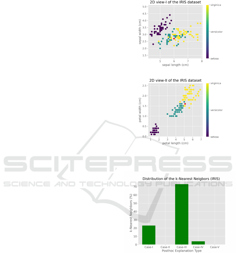
in Section 3.2. To examine this issue a little more,

we plotted 2D views of IRIS dataset as seen in Figure

4. Figure 4a shows 2D view of IRIS data from the

perspective of the attribute pair of “sepal width” and

“sepal length”, where the mispredicted sample, which

is normally belong to the category of “versicolor”, is

colored red. It is seen from Figure 4a that the mis-

predicted sample is located among “versicolor” and

“virginica” samples that makes it difﬁcult to distin-

guish. On the other hand, Figure 4b shows 2D view

of IRIS data from the perspective of the attribute pair

of “petal width” and “petal length”, where the mispre-

dicted sample is again colored red. It is seen from Fig-

ure 4b that the mispredicted sample is located near the

boundary between “versicolor” and “virginica” sam-

ples, which makes it clear why the model made in-

accurate prediction on this speciﬁc sample. This is

compatible with our posthoc analysis and interpreta-

tions that we have done above.

4.1.2 Statistical Analysis

In our experiments, 2 test samples out of 50 were mis-

predicted by the model, one of which have been ex-

plained in the previous part. In this part, we provide

statistical distribution of k-nearest neighbors based

posthoc analysis of these two mispredicted test sam-

ples. Figure 5 shows distribution as percentage of

the 11-nearest neighbors of the two mispredicted test

samples according to the cases in our posthoc analy-

sis. As seen in Figure 5, the majority of the 11-nearest

neighbors fall into Case-III, which implies that the

mispredicted test samples are either outliers or located

near boudaries.

4.2 CIFAR10 Dataset

The CIFAR-10 dataset consists of 60000 32x32

colour images in 10 different classes, with 6000 im-

ages per class, which are splitted as 50000:10000 for

training and test purposes. The 10 classes in CIFAR-

10 represent airplanes, cars, birds, cats, deer, dogs,

frogs, horses, ships, and trucks.

(a)

(b)

Figure 4: 2D views of IRIS dataset based on pairs of at-

tributes. The red circle represents the mispredicted sample

which is normally belong to category of “versicolor”.

Figure 5: Distribution of the 11-nearest neighbours of the

training set corresponding to inaccurate test samples when

they are given as input to the model.

In our experimental analysis, we implemented a CNN

which has similar architecture with VGG as follows:

Two successive 2D convolutional layers with 32 ﬁl-

ters and kernel size of (3,3), followed by pooling layer

and ﬂatten layer. Then a dense layer with 128 neu-

rons followed by a droput layer and ﬁnally ﬁnal dense

layer with softmax function. We trained the model up

to the optimal epoch where minimum validation loss

Explaining Inaccurate Predictions of Models through k-Nearest Neighbors

233

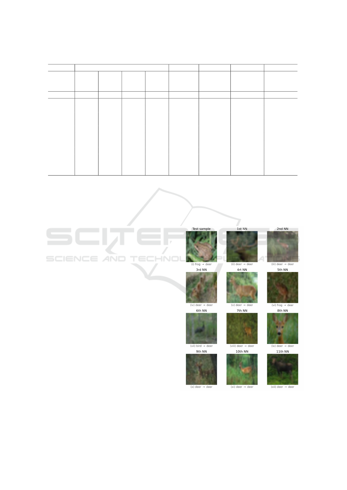
Table 3: 11-nearest neighbours of a sample based on euclidean distance in IRIS dataset.

Instance Attributes Distance Prediction True Label Explanation

Type sepal

length

(cm)

sepal

width

(cm)

petal

length

(cm)

petal

width

(cm)

euclidean

(cm)

Test 6.0 2.7 5.1 1.6 - virginica versicolor

NN 6.3 2.8 5.1 1.5 0.450 versicolor virginica Case IV

NN 6.3 2.7 4.9 1.8 0.462 virginica virginica Case III

NN 5.8 2.7 5.1 1.9 0.463 virginica virginica Case III

NN 6.3 2.5 4.9 1.5 0.612 versicolor versicolor Case I

NN 6.4 2.7 5.3 1.9 0.635 virginica virginica Case III

NN 5.7 2.8 4.5 1.3 0.676 versicolor versicolor Case I

NN 6.3 2.9 5.6 1.8 0.703 virginica virginica Case III

NN 6.3 2.5 5.0 1.9 0.709 virginica virginica Case III

NN 5.9 3.0 5.1 1.8 0.749 virginica virginica Case III

NN 6.0 3.0 4.8 1.8 0.758 virginica virginica Case III

is achieved, which allows us to avoid underﬁtting or

overﬁtting situations.

4.2.1 Sample-based Analysis

After completing the model training, we performed

predictions on test dataset, and picked an inaccurate

prediction for post-hoc analysis. Figure 6 shows the

mispredicted test sample along with its 11-nearest

neighbours from training dataset. The caption under

each subﬁgure indicates true label of the given ﬁgure

and the model’s prediction when this image is given

as input.

As seen in Figure 6, the original test image con-

tains a frog, but the model inaccurately classiﬁed this

sample as an deer image. When we look at the 11-

nearest neighbours, 1st, 2nd, 3rd, 4rt, 7th, 8th, 9th,

10th and 11th nearest neigbours (9 out of 11) fall into

Case III according to explanations given in Section

3.2, which implies that the model behaved in harmony

with the nearest neighbors for this speciﬁc test sam-

ple.

4.2.2 Statistical Analysis

In our experiments, the validation accuracy of the

model was about 68.61%, which corresponds to 3139

inaccurate predictions given that there are 10000 test

instances in CIFAR10 datasets. Taking k=3 in k-

nearest neighbors, we ﬁnd k-nearest neighbors for

all mispredicted test instances, and then performed

posthoc analysis according to explanations given in

Section 3.2. Figure 7 shows statistical distribution of

k-nearest neighbors according to the cases given in

our posthoc analysis.

As seen in Figure 7, almost 50% of the k-nearest

neighbors fall into Case-III, which implies that the

mispredicted test instances are likely to be outliers or

located near the boundaries of data points.

Figure 6: The 11-nearest neighbours in the training set for

a mispredicted test sample based on euclidean distance on

the extracted features at the internal layers of the neural net-

work.

ICAART 2021 - 13th International Conference on Agents and Artiﬁcial Intelligence

234

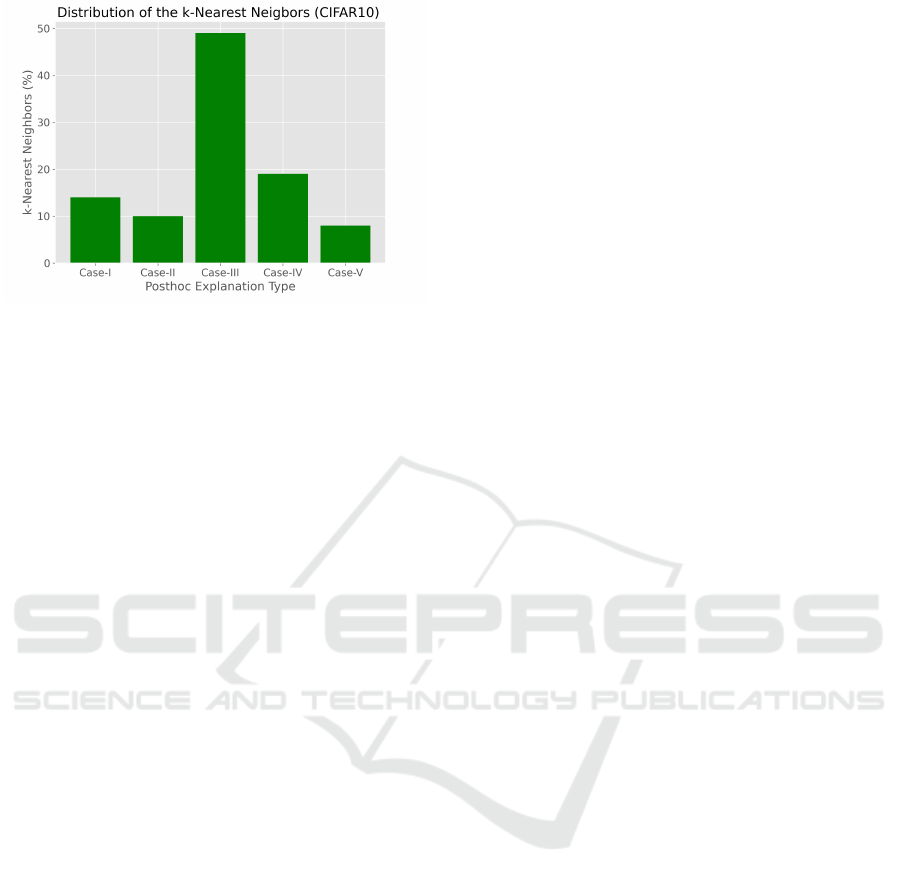
Figure 7: Distribution of the 3-nearest neighbours of the

training set corresponding to inaccurate test samples when

they are given as input to the model.

5 CONCLUSION

We studied the root causes of inaccurate decisions

reached particularly by deep learning models, which

is an important issue for many use cases that require

responsibility for the actions taken by AI. We devel-

oped a method for ﬁnding k-nearest neighbours in

training set for a given test instance, which were en-

hanced for ﬁnding similar images such that we calcu-

late euclidean distance not directly on the compared

images, but instead, on the features extracted from in-

ternal layers of the convolutional neural network. To

reveal possible root cause of an inaccurate prediction,

we thus ﬁnd k-nearest neighbours from training sam-

ples and re-entered them into the model to observe

its behaviour for further analysis. By comparing the

model’s responses on the k-nearest neighbours and

the associated test input, we estimated possible root

cause of the mispredictions. We validated our pro-

posed method on both IRIS and CIFAR-10 datasets,

and experimentally showed that our proposed method

can be used to understand why a model makes inac-

curate misprediction.

REFERENCES

Arrieta, A. B., D

ıaz-Rodr

ıguez, N., Del Ser, J., Bennetot,

A., Tabik, S., Barbado, A., Garc

ıa, S., Gil-L

opez, S.,

Molina, D., Benjamins, R., et al. (2020). Explainable

artiﬁcial intelligence (xai): Concepts, taxonomies, op-

portunities and challenges toward responsible ai. In-

formation Fusion, 58:82–115.

Barbado, A. and Corcho,

O. (2019). Rule extraction in

unsupervised anomaly detection for model explain-

ability: Application to oneclass svm. arXiv preprint

arXiv:1911.09315.

Bien, J. and Tibshirani, R. (2011). Prototype selection for

interpretable classiﬁcation. The Annals of Applied

Statistics, pages 2403–2424.

Bilgin, Z., Ersoy, M. A., Soykan, E. U., Tomur, E., C¸ omak,

P., and Karac¸ay, L. (2020). Vulnerability prediction

from source code using machine learning. IEEE Ac-

cess, 8:150672–150684.

Bologna, G. (2019). A simple convolutional neural network

with rule extraction. Applied Sciences, 9(12):2411.

Bologna, G. and Fossati, S. (2020). A two-step rule-

extraction technique for a cnn. Electronics, 9(6):990.

Bologna, G. and Hayashi, Y. (2017). Characterization of

symbolic rules embedded in deep dimlp networks: a

challenge to transparency of deep learning. Journal of

Artiﬁcial Intelligence and Soft Computing Research,

7(4):265–286.

Caruana, R., Kangarloo, H., Dionisio, J., Sinha, U., and

Johnson, D. (1999). Case-based explanation of non-

case-based learning methods. In Proceedings of the

AMIA Symposium, page 212. American Medical In-

formatics Association.

Castelvecchi, D. (2016). Can we open the black box of ai?

Nature News, 538(7623):20.

Chakraborti, T., Sreedharan, S., and Kambhampati, S.

(2020). The emerging landscape of explainable

ai planning and decision making. arXiv preprint

arXiv:2002.11697.

Cui, X., Lee, J. M., and Hsieh, J. (2019). An integrative 3c

evaluation framework for explainable artiﬁcial intelli-

gence.

Dua, D. and Graff, C. (2017). UCI machine learning repos-

itory.

Fisher, R. A. (1936). The use of multiple measurements in

taxonomic problems. Annals of eugenics, 7(2):179–

188.

Goodman, B. and Flaxman, S. (2017). European union reg-

ulations on algorithmic decision-making and a “right

to explanation”. AI magazine, 38(3):50–57.

Gunning, D. and Aha, D. W. (2019). Darpa’s explainable ar-

tiﬁcial intelligence program. AI Magazine, 40(2):44–

58.

Hall, P. (2018). On the art and science of machine learning

explanations. arXiv preprint arXiv:1810.02909.

Hendricks, L. A., Akata, Z., Rohrbach, M., Donahue, J.,

Schiele, B., and Darrell, T. (2016). Generating visual

explanations. In European Conference on Computer

Vision, pages 3–19. Springer.

Holzinger, A., Langs, G., Denk, H., Zatloukal, K., and

uller, H. (2019). Causability and explainability of

artiﬁcial intelligence in medicine. Wiley Interdisci-

plinary Reviews: Data Mining and Knowledge Dis-

covery, 9(4):e1312.

Krizhevsky, A., Hinton, G., et al. (2009). Learning multiple

layers of features from tiny images.

Li, O., Liu, H., Chen, C., and Rudin, C. (2018). Deep learn-

ing for case-based reasoning through prototypes: A

neural network that explains its predictions. In Thirty-

second AAAI conference on artiﬁcial intelligence.

Lipton, Z. C. (2018). The mythos of model interpretability.

Queue, 16(3):31–57.

Explaining Inaccurate Predictions of Models through k-Nearest Neighbors

235

Papernot, N. and McDaniel, P. (2018). Deep k-nearest

neighbors: Towards conﬁdent, interpretable and ro-

bust deep learning. arXiv preprint arXiv:1803.04765.

Pedregosa, F., Varoquaux, G., Gramfort, A., Michel, V.,

Thirion, B., Grisel, O., Blondel, M., Prettenhofer,

P., Weiss, R., Dubourg, V., Vanderplas, J., Passos,

A., Cournapeau, D., Brucher, M., Perrot, M., and

Duchesnay, E. (2011). Scikit-learn: Machine learning

in Python. Journal of Machine Learning Research,

12:2825–2830.

Petkovic, D., Altman, R. B., Wong, M., and Vigil, A.

(2018). Improving the explainability of random for-

est classiﬁer-user centered approach. In PSB, pages

204–215. World Scientiﬁc.

Ribeiro, M. T., Singh, S., and Guestrin, C. (2016). ” why

should i trust you?” explaining the predictions of any

classiﬁer. In Proceedings of the 22nd ACM SIGKDD

international conference on knowledge discovery and

data mining, pages 1135–1144.

Roscher, R., Bohn, B., Duarte, M. F., and Garcke, J. (2020).

Explainable machine learning for scientiﬁc insights

and discoveries. IEEE Access, 8:42200–42216.

Tjoa, E. and Guan, C. (2019). A survey on explainable ar-

tiﬁcial intelligence (xai): towards medical xai. arXiv

preprint arXiv:1907.07374.

Ustundag Soykan, E., Bilgin, Z., Ersoy, M. A., and Tomur,

E. (2019). Differentially private deep learning for load

forecasting on smart grid. In 2019 IEEE Globecom

Workshops (GC Wkshps), pages 1–6.

ICAART 2021 - 13th International Conference on Agents and Artiﬁcial Intelligence

236