
Classification of Normal versus Leukemic Cells with Data Augmentation
and Convolutional Neural Networks
Jos
´
e Elwyslan Maur
´
ıcio de Oliveira
a
and Daniel Oliveira Dantas
b
Departamento de Computac¸
˜
ao, Universidade Federal de Sergipe, S
˜
ao Crist
´
ov
˜
ao, SE, Brazil
Keywords:
Leukemia Classification, Acute Lymphoblastic Leukemia.
Abstract:
Acute lymphoblastic leukemia is the most common childhood leukemia. It is an aggressive cancer type and
causes various health problems. Diagnosis depends on manual microscopic analysis of blood samples by
expert hematologists and pathologists. To assist these professionals, image processing and pattern recognition
techniques can be used. This work proposes simple modifications to standard neural network architectures
to achieve high performance in the malignant leukocyte classification problem. The tested architectures were
VGG16, VGG19 and Xception. Data augmentation was employed to balance the Training and Validation
sets. Transformations such as mirroring, rotation, blurring, shearing, and addition of salt and pepper noise
were used. The proposed method achieved an F1-score of 92.60%, the highest one when compared to other
participants’ published results and eighth position when compared to the weighted F1-score provided by the
competition leaderboard.
1 INTRODUCTION
Blood is a connective tissue that flows within the
blood vessels of animals that have a closed circula-
tory system. In hematology, the branch of medicine
concerned with the study of blood, changes in the
shape and function of leukocytes are called leukocyte
abnormalities, and leukemia is one of those abnor-
malities. These abnormalities are defined by the ac-
cumulation of myeloblasts (immature granulocytes)
or lymphoblasts (immature lymphocytes) in the bone
marrow and peripheral blood. Leukemia can occur in
two forms: acute or chronic. Acute leukemia is the
most aggressive since it evolves rapidly and presents
its symptoms more intensely than the chronic version.
Acute Lymphoblastic Leukemia (ALL), the main
object of this study, occurs when a large number of
lymphoblasts accumulate in the bone marrow and pe-
ripheral blood. These immature lymphocytes do not
differentiate into their mature forms, causing health
problems such as infections or cancer. ALL is the
most common childhood leukemia. The highest oc-
currence of ALL being in children between 3 and 7
years old with 75% of diagnoses occurring before the
age of 6. Of these diagnoses, 85% are from leukemias
a
https://orcid.org/0000-0002-0282-0921
b
https://orcid.org/0000-0002-0142-891X
that affect B type lymphocytes (ALL-B) (Hoffbrand
and Moss, 2013).
Manual microscopic analysis of blood samples is
the primary method for analyzing lymphocytes ex-
tracted from patients with leukemia. As a result, the
classification of healthy and malignant lymphocytes
highly depends upon the expertise of the hematolo-
gists and pathologists in recognizing the two classes.
To assist these professionals in live blood analysis,
image processing and pattern recognition techniques
have been extensively used to produce Computer-
Aided Diagnosis (CADx) systems. These systems
aim to increase the accuracy of lymphocyte classifi-
cation (Mishra et al., 2019; Moshavash et al., 2018).
The Acute Lymphoblastic Leukemia Image
Database (ALL-IDB) (Labati et al., 2011; DI-UNIMI,
2020) for Image Processing is a public and free
dataset of microscopic images of blood samples for
the evaluation of segmentation and image classifica-
tion algorithms focusing on ALL. The ALL-IDB ini-
tiative provides two different datasets: ALL-IDB1,
which consists of 108 blood smear images collected
from healthy and leukemic patients, containing 510
single leukocytes; and ALL-IDB2 which is a col-
lection of the cropped areas of interest of normal
and malignant leukocytes that belong to the ALL-
IDB1 dataset. Samples of both ALL-IDB datasets are
shown in Figure 1.
Maurício de Oliveira, J. and Dantas, D.
Classification of Normal versus Leukemic Cells with Data Augmentation and Convolutional Neural Networks.
DOI: 10.5220/0010257406850692
In Proceedings of the 16th International Joint Conference on Computer Vision, Imaging and Computer Graphics Theory and Applications (VISIGRAPP 2021) - Volume 4: VISAPP, pages
685-692
ISBN: 978-989-758-488-6
Copyright
c
2021 by SCITEPRESS – Science and Technology Publications, Lda. All rights reserved
685
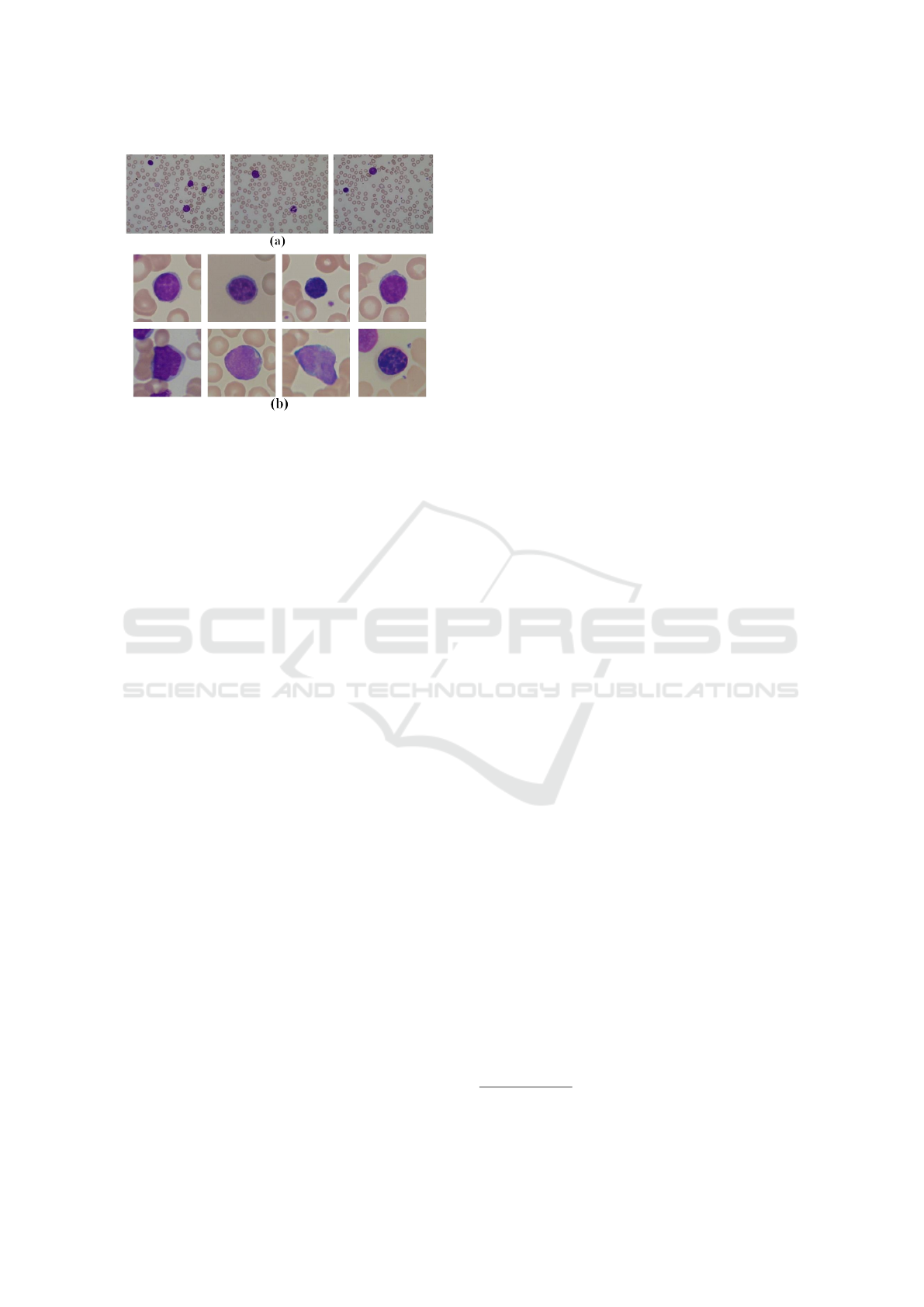
Figure 1: ALL-IDB image samples (DI-UNIMI, 2020): (a)
ALL-IDB1 and (b) ALL-IDB2.
Many works in the literature use small datasets.
Usage of the dataset ALL-IDB, which contains
only 510 lymphocytes, was commonplace, and
many feature extraction based approaches were pro-
posed (Putzu et al., 2014; MoradiAmin et al., 2016;
Mishra et al., 2016; Rawat et al., 2017; Moshavash
et al., 2018). However, most current works use con-
volutional neural networks (CNN) to address the lym-
phocyte classification task.
Shafique and Tehsin (Shafique and Tehsin, 2018)
deployed a pretrained AlexNet for detection and clas-
sification of ALL lymphocytes. ALL-IDB2 dataset
was used in combination with data augmentation to
increase the number of training samples by apply-
ing image rotation and mirroring in the source im-
ages. The training data was increased from 260 im-
ages to 760, where 500 are malignant samples and
260 healthy samples. The augmented dataset was di-
vided into training data and test data in a 6:4 ratio.
The pretrained AlexNet achieved an overall accuracy
of 99.50%.
Rehman et al. (Rehman et al., 2018) also propose
a deep learning solution using Alexnet and transfer
learning. In his work, only the top layers of Alexnet
were modified and fine-tuned. ALL-IDB was used
without data augmentation. The test set contained
330 images, and the network achieved an accuracy of
97.78%.
Ahmed et al. (Ahmed et al., 2019) conducted
some experiments with ALL-IDB, in one of which
they had develop their own CNN architecture. Data
augmentation was used to balance and expand the
dataset. The training was performed with 980 sam-
ples, and an additional 245 samples were used as test,
with both sets being balanced. His CNN achieved an
accuracy of 88.5%.
Recent initiatives have released large datasets to
train and evaluate leukemia cell classifiers. One is the
CNMC-2019 dataset created by the SBILab (SBILab,
2020) research team. This dataset is used in this work
and is detailed in Subsection 2.1.
Mourya et al. (Mourya et al., 2018) (SBILab
members) introduced a deep learning framework for
classifying malignant and healthy lymphocytes that
combine discrete cosine transform (DCT) features
and convolutional neural networks (CNN) in a hybrid
architecture called Leukonet. They have prepared a
dataset of 9211 cancer cells from 65 subjects and
4528 healthy cells from 52 subjects, which together
composed the training data of 13739 cells, divided
into four sets for cross-validation. The test data used
to evaluate Leukonet consist of 312 cancer cells and
324 healthy cells. Its hybrid architecture achieved an
accuracy of 89.70% and an F1-score of 91.95% for
cancer cell class.
In 2019 the SBILab hosted a competition in which
participants are to make use of the C-NMC 2019
Dataset to propose classification methods for ALL-B
cells into healthy or malignant. At the end of the com-
petition, winning approaches were published (Gupta
and Gupta, 2019). All submitted solutions were based
on convolutional neural networks, and many had large
and complex architectures. We show throughout this
paper that it is possible to achieve a high score in this
challenge using slightly modified traditional architec-
tures and standard training methods.
This article is organized as follows: Section 2 de-
scribes the methodology used in this work; Section 3
presents the obtained results, and; the conclusions are
given in Section 4.
2 METHODOLOGY
In this work, images of healthy and malignant lym-
phocytes from C-NMC 2019 Dataset were used for
training variations of the Xception and VGGNet ar-
chitectures, in order to create a classifier capable of
distinguishing the two cell types. These architectures
were fine-tuned so that the models achieved the high-
est validation accuracy possible. In the end, the best
models of each architecture had their performances
evaluated in the Test set.
The implementation of this methodology is pub-
licly available
1
and was coded in Python using Ten-
sorflow, Keras, Numpy, SciPy and OpenCV.
1
https://github.com/Elwyslan/ISBI-2019-Cells-
Classification/tree/master/classifiers/10.ConvolutionalNets
VISAPP 2021 - 16th International Conference on Computer Vision Theory and Applications
686
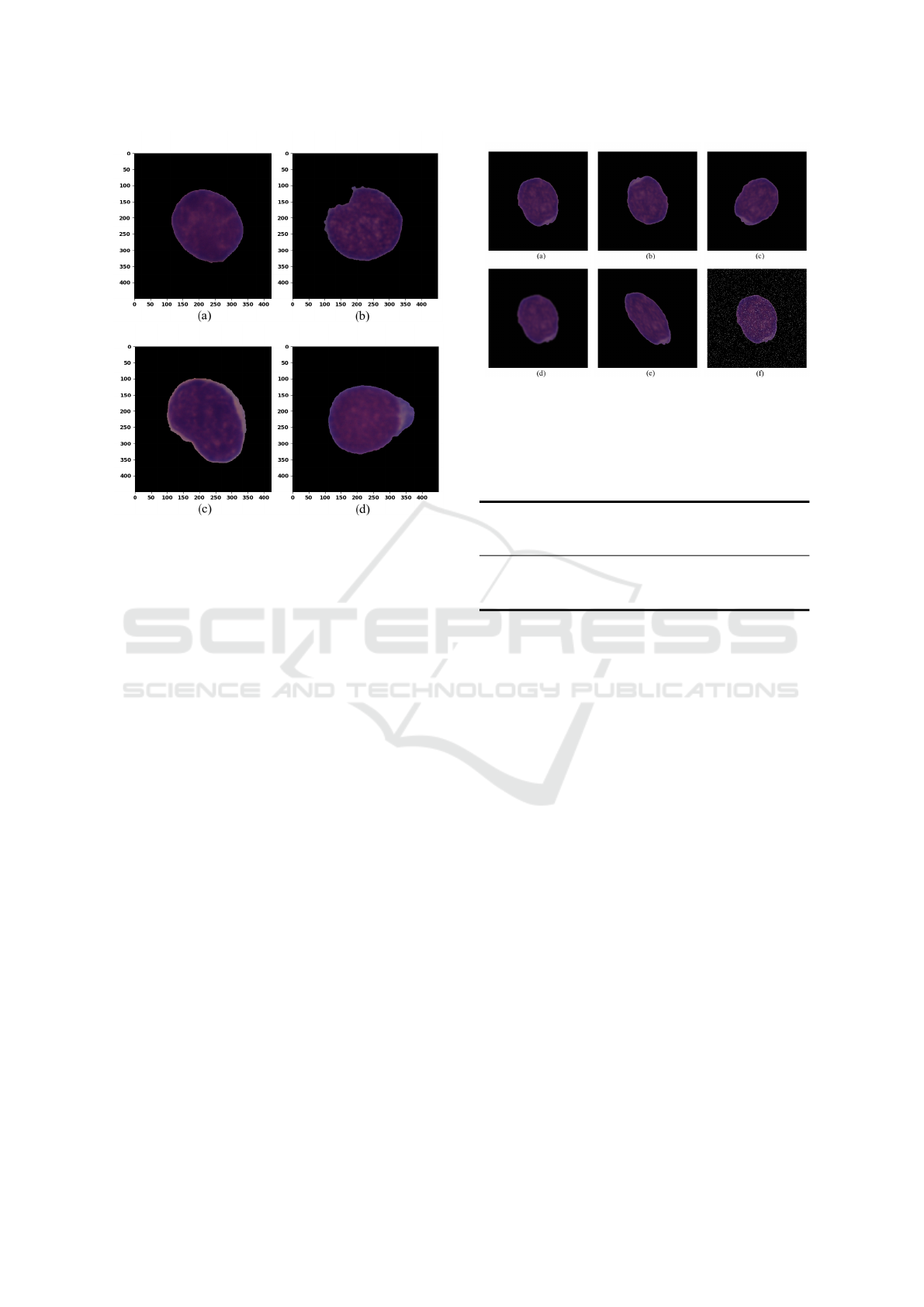
Figure 2: C-NMC 2019 Dataset samples. (a) and (c) are ma-
lignant lymphocytes, (b) and (d) are healthy lymphocytes.
2.1 C-NMC 2019 Dataset
The SBILab (SBILab, 2020) research team was
responsible for creating and publishing the image
dataset used in this work. They performed all the
steps related to image preprocessing, image enhance-
ment, lymphocyte segmentation, and stain normaliza-
tion using standard image processing techniques and
inhouse methods (Duggal et al., 2016; Gupta et al.,
2017; Duggal et al., 2017).
The C-NMC 2019 Dataset, publicly avail-
able (Mourya et al., 2019), consists of 15114 lym-
phocyte images collected from 118 subjects and split
into three folders with names: “C-NMC training data”
containing 10661 cells, 7272 malignant cells from 47
subjects and 3389 healthy cells from 26 subjects; “C-
NMC test preliminary phase data” containing 1867
cells, 1219 malignant cells from 13 subjects and 648
healthy cells from 15 subjects, and “C-NMC test fi-
nal phase data” containing 2586 unlabeled cells from
17 subjects. Within these folders, there are single cell
images of malignant and healthy lymphocytes previ-
ously labeled by expert oncologists.
Cells had been dyed using Jenner-Giemsa stain
technique (Marzahl et al., 2019), and the images were
stain-normalized before the segmentation. The blood
smear image is a bitmap RGB with 24 bits color
depth and size of 2560x1920 pixels. The lymphocytes
were segmented from each of the blood smear images
and placed in the center of individual images of size
450×450 pixels with a black background. Figure 2
Figure 3: Examples of augmented images: (a) source im-
age; (b) vertical and horizontal mirroring; (c) clockwise
rotation by 60
◦
; (d) Gaussian blur with 17×17 kernel; (e)
shearing with a factor of 0.3, and; (f) salt and pepper noise.
Table 1: Number of samples in Training, Validation and
Test sets.
Before
Data Augmentation
After
Data Augmentation
Malignant Healthy Malignant Healthy
Training
4364 2034 10000 10000
Validation
2181 1016 5000 5000
Test
727 339 N/A N/A
shows samples of malignant and healthy lymphocytes
of the C-NMC 2019 Dataset.
The unlabeled data in the C-NMC test final phase
data is used to evaluate the medical image classifica-
tion challenge entitled “C-NMC challenge: Classifi-
cation of Normal versus Malignant Cells in B-ALL
White Blood Cancer Microscopic Images” organized
by SBILab (SBILab, 2019a). The participants in this
challenge can evaluate their results on C-NMC test
final phase data by submitting it to the leaderboard
hosted on competition website.
In this work, the “C-NMC training data” was used,
whose images were randomly split into Training, Val-
idation, and Test sets in a 6:3:1 ratio. The division
of the 7272 malignant lymphocytes was as follows:
4364 were for the Training set, 2181 for the Valida-
tion set, and 727 for the Test set. Regarding the 3389
healthy lymphocytes: 2034 were for the Training set,
1016 for the Validation set and 339 for the Test set.
The split is shown in Table 1.
2.2 Data Augmentation
The original dataset was unbalanced and, for that rea-
son, data augmentation was employed to balance the
Training and Validation sets. This technique was not
applied to the Test set. Standard image transforma-
tion techniques were used, such as mirroring, rotation,
Classification of Normal versus Leukemic Cells with Data Augmentation and Convolutional Neural Networks
687

and Gaussian blurring, to produce the augmented im-
ages. We also attempted different augmentation tech-
niques, and it was noticed that shearing and addition
of salt and pepper noise resulted in a better train-
ing performance and model accuracy. An example
of these techniques applied to a random image from
the dataset can be seen in Figure 3. The augmented
Training set had 20,000 samples, and the Validation
set has 10,000 samples, as shown in Table 1.
2.3 Convolutional Neural Network
Classifier
The VGG16, VGG19, and Xception architectures
were chosen to build the classifiers. The Xcep-
tion (Chollet, 2017) and VGGNet (Simonyan and Zis-
serman, 2014) were the best qualified CNN archi-
tectures presented in the ImageNet Large Scale Vi-
sual Recognition Challenge (ILSVRC) (Russakovsky
et al., 2015; Dhillon and Verma, 2019).
The VGGNet, proposed by the Visual Geometry
Group (VGG) from Oxford University, has six dif-
ferent convolutional network configurations by the
names of: VGG11, VGG11-LRN, VGG13, VGG16
(Conv1), VGG16, and VGG19. Each of these config-
urations has the number of convolutional layers equal
to the number associated with its name. In ILSVRC,
VGG16 and VGG19 achieved the highest accuracy.
The VGG16 and VGG19 top layers consist of a
global max pooling layer followed by two fully con-
nected layers with 4096 neurons using ReLU activa-
tion function. The output layer is made of 1000 neu-
rons using softmax function. In our work, these layers
were replaced by a global average pooling layer fol-
lowed by two fully connected layers with 512 neurons
using ReLU, then linked to a prediction layer with two
neurons using softmax function.
The Xception extends the concept of performing
several convolutions with different filter sizes from
Inception’s module by using the concept of depthwise
separable convolutions. This architecture is com-
posed of 36 depthwise separable convolution layers,
structured in 14 modules. The modules have residual
connections to each other, except for the first and last
modules (Chollet, 2017).
The Xception top layers consist of a global av-
erage pooling layer which produces a 1×2048 vec-
tor. In the paper that describes the architecture, Chol-
let (Chollet, 2017) does not specify any fully con-
nected or prediction layer, therefore we decided to
place one fully connected layer with 2048 neurons us-
ing ReLU linked to 2 neurons using softmax.
The first paper to propose Global Average Pooling
(GAP) layers (Lin et al., 2013) introduces the idea of
taking the average of each feature map and feeding
the resulting vector directly into the softmax layer in-
stead of adding fully connected layers on top of the
convolutional neural network. However, in our exper-
iments, the addition of a few more layers after GAP
produced a slight increase in validation accuracy com-
pared to the same setup using max pooling layers. The
VGGNet and Xception were designed to classify im-
ages into 1000 different classes, while our problem
involves only two classes. With few classes, it is pos-
sible to reduce the number of neurons in each fully
connected layer without any decrease in model accu-
racy.
A Dropout (Hinton et al., 2012a) layer was in-
cluded, following each neuron layer, with a fixed
dropout rate of 50%. The only exception was the out-
put layer. A dropout rate of 50% means randomly dis-
abling half of the neuron connections in every train-
ing batch. This approach helps to prevent overfitting
and complex co-adaptations on training data (Hinton
et al., 2012b).
The output layer is composed of two neurons that
use softmax activation function. The main property
of softmax is to produce a distribution of probabilities
in the output of the neural network based on neuron
logits. The softmax function is given by equation 1:
softmax(z
i
) =
e
z
i
K
∑
j=1
e
z
j
(1)
where z
i
is the vector formed by the K logits of the
output layer.
Figure 4 shows a summary of the top layers of the
three architectures.
2.4 Image Normalization
The lymphocytes present in the images have a major
axis of 223 ± 43 pixels on average. Due to this at-
tribute, we decided to crop 100 pixels from each bor-
der, reducing the original image size from 450×450
to 250×250. By performing this operation, it was
possible to reduce the image size without losing sub-
stantial cell area and to avoid resizing algorithms. Af-
ter cropping, the pixels were converted to float by di-
viding their values by 255.0, and the channel mean
value was subtracted.
2.5 Training
All training was done in a virtual machine from
Google Cloud Platform with an Intel Core i5 2.40
GHz, 20 GB of RAM, and an NVIDIA Tesla T4
graphic card.
VISAPP 2021 - 16th International Conference on Computer Vision Theory and Applications
688
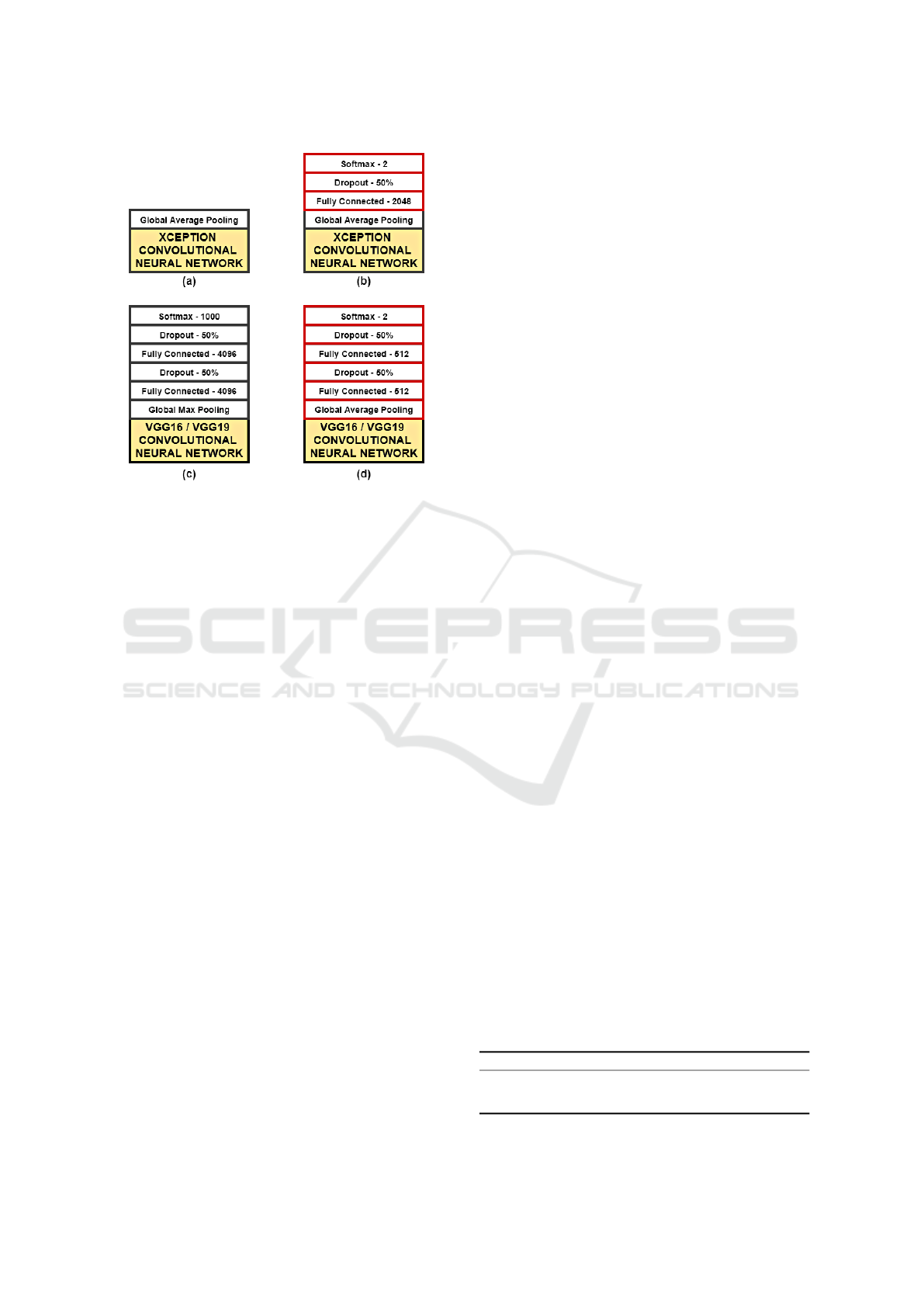
Figure 4: Top layers of the convolutional networks used in
this work: (a) original Xception top layers; (b) Xception
variant used in our work; (c) Original VGG16 and VGG19
top layers, and; (d) VGG16 and VGG19 variants used in our
work.
Along with softmax, the binary cross-entropy loss
was utilized. Cross-entropy loss measures the similar-
ity of a classification model that outputs a probability
value between 0 and 1 for each class. This loss pe-
nalizes divergence of the predicted probability q from
its target probability distribution p as defined in Equa-
tion 2. The loss was optimized using Adam with the
same hyperparameter values proposed by Kingma and
Ba (Kingma and Ba, 2014).
H(p, q) = −
∑
i
p
i
log(q
i
) (2)
We applied a regularization term only to the fully-
connected layers. The regularization term is com-
posed of L
1
and L
2
norms. The L
1
regularization is
the sum of the absolute values of the weight matrix
of the neuron layer, and L
2
regularization is the sum
of all squared weight values of the same matrix. We
combine these two norms into a single regularization
term, λ, to simplify the fine-tuning process. The fully-
connected network loss can be rewritten as in Equa-
tion 3:
Loss = Cross-Entropy+λ
L
1
∑
i
|
W
i
|
+ λ
L
2
∑
i
W
2
i
Loss = Cross-Entropy+λ
∑
i
|
W
i
|
+
∑
i
W
2
i
!
(3)
where W
i
is the layer weight matrix with coefficients
i, λ
L
1
λ
L
2
are L
1
and L
2
regularization terms respec-
tively and λ = λ
L
1
= λ
L
2
. The regularization term λ
was adjusted in order to obtain the lowest validation
loss.
A learning rate schedule was also used, with initial
and final learning rates that exponentially decay over
400 epochs. Their values were chosen to make the
training process of each CNN stable.
3 RESULTS AND DISCUSSION
The Test dataset is unbalanced, which can result in
misleading accuracy. To evaluate the performance of
the classifiers, the primary metric used was the F1-
score. An advantage of the F1-score is the possi-
bility of comparing our results with those obtained
by the teams that participated in SBILab’s challenge,
which have used the same dataset and also use the
F1-score as the evaluation metric for ranking pur-
poses. The results can be found in a book published
by Gupta (Gupta and Gupta, 2019).
The accuracy, precision, sensitivity (also known
as recall), and specificity obtained by the best per-
forming convolutional neural networks when applied
to the Test set are shown in Table 2.
In this study, the best model achieved an F1-
score of 92.60%, precision of 91.14%, sensitivity of
94.10%, and specificity of 90.86% for the malignant
class. This result was obtained with a VGG16 net-
work using as the prediction stage the following se-
quence of layers: one GAP layer, a fully connected
layer with 512 neurons using ReLU, a 50% dropout
layer, another fully connected layer with 512 neurons
using ReLU, another 50% dropout layer and, on the
top, a two-neuron layer using softmax, as shown in
Figure 4(d). The network was trained from scratch.
A learning rate schedule was also used, with an ini-
tial learning rate of 0.00001 exponentially decaying
to 0.000001 over 400 epochs. The regularization term
λ was set to 0.0001. The validation and training accu-
racies are shown in Figure 5.
The first runner-up achieved an F1-score of
91.75%, a precision of 90.06%, a sensitivity of
93.51%, and a specificity of 86.68% for the malignant
class. This result was obtained by a VGG19 network
using the same setup as in the VGG16. The validation
and training accuracy during the training are shown in
Figure 6.
Table 2: Performance of the trained Convolutional Neural
Network architectures in Test set.
Accuracy Precision Sensitivity Specificity F1-Score
VGG16 92.48% 91.14% 94.10% 90.86% 92.60%
VGG19 91.59% 90.06% 93.51% 86.68% 91.75%
Xception 90.41% 87.64% 94.10% 86.73% 90.76%
Classification of Normal versus Leukemic Cells with Data Augmentation and Convolutional Neural Networks
689
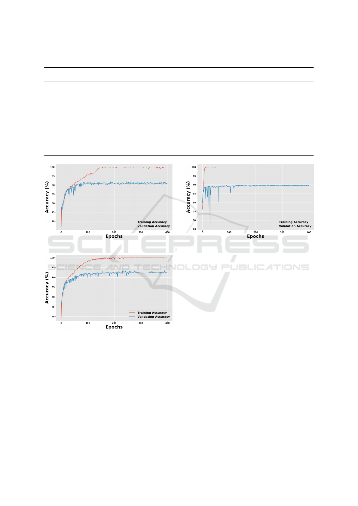
Table 3: Performance of participants in C-NMC challenge hosted by SBILab.
Participant in
SBILab challenge
F1-score Methodology
Our model
92.60%
Train a VGG16 architecture from scratch
(Pan et al., 2019)
92.50%
Transfer learning Resnets in a neighborhood-correction algorithm
(Honnalgere and Nayak, 2019)
91.70%
Transfer learning with a VGG16 architecture
(Xiao et al., 2019)
90.30%
Deep multi-model ensemble network (various convolutional neural networks)
(Verma and Singh, 2019)
89.47%
Transfer learning with a MobileNetV2 architecture
(Prellberg and Kramer, 2019)
87.89%
Training from scratch a ResNeXt50 architecture
(Shah et al., 2019)
87.58%
Transfer learning with a combination of convolutional and recurrent neural networks
(Marzahl et al., 2019)
87.46%
Transfer learning with a ResNet18 architecture
(Ding et al., 2019)
86.74%
Training from scratch InceptionV3, DenseNet and InceptionResNetV2 architectures
(Kulhalli et al., 2019)
85.70%
Training from scratch ResNeXt50 and ResNeXt101 architectures
(Liu and Long, 2019)
84.00%
Transfer learning with Inception and ResNets architectures
(Khan and Choo, 2019)
81.79%
Transfer learning with ResNets and SENets
Figure 5: VGG16 training.
Figure 6: VGG19 training.
The second runner-up achieved an F1-score of
90.76%, a precision of 87.64%, a sensitivity of
94.10%, and a specificity of 86.73% for the malig-
nant class. This result was obtained by an Xception
network using as a prediction stage the following se-
quence of layers: one GAP layer, a fully connected
layer with 2048 neurons using ReLU, a 50% dropout
layer, and, on the top, a two-neuron layer using soft-
max, as shown in Figure 4(b). The network was again
trained from scratch with a learning rate schedule
with an initial learning rate of 0.000005 exponentially
decaying to 0.000001 over 400 epochs. The regular-
ization term λ was set to 0.0007. The validation and
Figure 7: Xception training.
training accuracies are shown in Figure 7.
Compared to the results in Table 3, we achieved a
top score result with our methodology using standard
neural network architectures with simple additions.
The F1-score shown in Table 3 published by the par-
ticipants were obtained by models trained and eval-
uated with images from “C-NMC training data” and
“C-NMC test preliminary phase data”. As mentioned
in Subsection 2.1, we used only “C-NMC training
data” to train and evaluate our models.
We evaluated the three models with the competi-
tion Test data, contained in “C-NMC test final phase
data”, by submitting the results to the competition
website. Since this dataset is unlabeled, we were un-
able to compute other performance metrics. The only
metric provided by the competition leaderboard is the
Weighted F1-Score. The results obtained by the three
models in the competition leaderboard are shown in
Table 4. The final result of ISBI 2019 challenge is
shown in Table 5.
The highest result, 86.35177019%, obtained by
the Xception model could place the proposed method-
ology in the 8th position on challenge’s ranking.
VISAPP 2021 - 16th International Conference on Computer Vision Theory and Applications
690

Table 4: Performance of CNN architectures in Competition
Leaderboard.
Architecture Weighted F1-Score
Xception 86.35177019%
VGG16 83.24786937%
VGG19 82.59010758%
Table 5: Top entries of C-NMC 2019 Challenge pub-
lished (SBILab, 2019b).
Name Rank Weighted F1-Score
Yongsheng Pan 1 0.910
Ekansh Verma 2 0.894
Jonas Prellberg 3 0.889
Fenrui Xiao 4 0.885
Tian Shi 5 0.879
Ying Liu 6 0.876
Salman Shah 7 0.866
Yifan Ding 8 0.855
Xinpeng Xie 9 0.848
4 CONCLUSIONS AND FUTURE
WORK
Our results indicate that the proposed methodology
based on a convolutional neural network is able to
classify lymphocyte images into malignant or healthy
with high accuracy. Simple modifications in conven-
tional CNN architectures were enough to create clas-
sifiers with results similar to complex methodologies.
In the literature, many methods were tested with
only a few sample images or with private datasets. On
the other hand, our study was done with a large and
public dataset. Therefore the result obtained is more
general and can easily be replicated.
An F1-score of 92.60% lacks confidence for dis-
ease diagnosis but can serve as a tool to assist on-
cologists. In conclusion, the proposed method in this
study is a technique with high performance in classifi-
cation of cancerous lymphocyte images which can be
used complementarily in immunophenotyping.
REFERENCES
Ahmed, N., Yigit, A., Isik, Z., and Alpkocak, A. (2019).
Identification of leukemia subtypes from microscopic
images using convolutional neural network. Diagnos-
tics, 9(3):104.
Chollet, F. (2017). Xception: Deep learning with depthwise
separable convolutions. In 2017 IEEE Conference
on Computer Vision and Pattern Recognition (CVPR).
IEEE.
Dhillon, A. and Verma, G. K. (2019). Convolutional neu-
ral network: a review of models, methodologies and
applications to object detection. Progress in Artificial
Intelligence, 9(2):85–112.
DI-UNIMI (2020). ALL-IDB: Acute Lymphoblastic
Leukemia Image Database for Image Processing.
https://homes.di.unimi.it/scotti/all/.
Ding, Y., Yang, Y., and Cui, Y. (2019). Deep learning for
classifying of white blood cancer. In Lecture Notes in
Bioengineering, pages 33–41. Springer Singapore.
Duggal, R., Gupta, A., Gupta, R., and Mallick, P. (2017).
SD-layer: Stain deconvolutional layer for CNNs
in medical microscopic imaging. In Medical Im-
age Computing and Computer Assisted Intervention -
MICCAI, pages 435–443. Springer International Pub-
lishing.
Duggal, R., Gupta, A., Gupta, R., Wadhwa, M., and
Ahuja, C. (2016). Overlapping cell nuclei segmen-
tation in microscopic images using deep belief net-
works. In Proceedings of the Tenth Indian Conference
on Computer Vision, Graphics and Image Processing
- ICVGIP. ACM Press.
Gupta, A. and Gupta, R., editors (2019). ISBI 2019 C-
NMC Challenge: Classification in Cancer Cell Imag-
ing. Springer Singapore.
Gupta, R., Mallick, P., Duggal, R., Gupta, A., and Sharma,
O. (2017). Stain color normalization and segmenta-
tion of plasma cells in microscopic images as a pre-
lude to development of computer assisted automated
disease diagnostic tool in multiple myeloma. Clinical
Lymphoma Myeloma and Leukemia, 17(1):e99.
Hinton, G. E., Krizhevsky, A., Sutskever, I., and Srivastva,
N. (2012a). System and method for addressing over-
fitting in a neural network. Patent US9406017B2 as-
signed to Google LLC.
Hinton, G. E., Srivastava, N., Krizhevsky, A., Sutskever, I.,
and Salakhutdinov, R. R. (2012b). Improving neural
networks by preventing co-adaptation of feature de-
tectors.
Hoffbrand, A. V. and Moss, P. A. H. (2013). Essential
Haematology. Wiley, New Jersey, USA, 6 edition.
Honnalgere, A. and Nayak, G. (2019). Classification of nor-
mal versus malignant cells in b-ALL white blood can-
cer microscopic images. In Lecture Notes in Bioengi-
neering, pages 1–12. Springer Singapore.
Khan, M. A. and Choo, J. (2019). Classification of can-
cer microscopic images via convolutional neural net-
works. In Lecture Notes in Bioengineering, pages
141–147. Springer Singapore.
Kingma, D. P. and Ba, J. (2014). Adam: A method for
stochastic optimization.
Kulhalli, R., Savadikar, C., and Garware, B. (2019). To-
ward automated classification of B-acute lymphoblas-
tic leukemia. In Lecture Notes in Bioengineering,
pages 63–72. Springer Singapore.
Labati, R. D., Piuri, V., and Scotti, F. (2011). ALL-IDB:
The Acute Lymphoblastic Leukemia Image Database
for Image Processing. In 18th IEEE International
Classification of Normal versus Leukemic Cells with Data Augmentation and Convolutional Neural Networks
691

Conference on Image Processing - ICIP, pages 2045–
2048. IEEE.
Lin, M., Chen, Q., and Yan, S. (2013). Network in network.
Liu, Y. and Long, F. (2019). Acute lymphoblastic leukemia
cells image analysis with deep bagging ensemble
learning. In Lecture Notes in Bioengineering, pages
113–121. Springer Singapore.
Marzahl, C., Aubreville, M., Voigt, J., and Maier, A. (2019).
Classification of leukemic b-lymphoblast cells from
blood smear microscopic images with an attention-
based deep learning method and advanced augmenta-
tion techniques. In Lecture Notes in Bioengineering,
pages 13–22. Springer Singapore.
Mishra, S., Majhi, B., and Sa, P. K. (2019). Texture feature
based classification on microscopic blood smear for
acute lymphoblastic leukemia detection. Biomedical
Signal Processing and Control, 47:303–311.
Mishra, S., Sharma, L., Majhi, B., and Sa, P. K. (2016).
Microscopic image classification using DCT for the
detection of acute lymphoblastic leukemia (ALL).
In Advances in Intelligent Systems and Computing,
pages 171–180. Springer Singapore.
MoradiAmin, M., Memari, A., Samadzadehaghdam, N.,
Kermani, S., and Talebi, A. (2016). Computer aided
detection and classification of acute lymphoblastic
leukemia cell subtypes based on microscopic im-
age analysis. Microscopy Research and Technique,
79(10):908–916.
Moshavash, Z., Danyali, H., and Helfroush, M. S. (2018).
An automatic and robust decision support system
for accurate acute leukemia diagnosis from blood
microscopic images. Journal of Digital Imaging,
31(5):702–717.
Mourya, S., Kant, S., Kumar, P., Gupta, A., and Gupta, R.
(2018). LeukoNet: DCT-based CNN architecture for
the classification of normal versus Leukemic blasts in
B-ALL Cancer.
Mourya, S., Kant, S., Kumar, P., Gupta, A., and Gupta, R.
(2019). ALL challenge dataset of ISBI.
Pan, Y., Liu, M., Xia, Y., and Shen, D. (2019).
Neighborhood-correction algorithm for classification
of normal and malignant cells. In Lecture Notes in
Bioengineering, pages 73–82. Springer Singapore.
Prellberg, J. and Kramer, O. (2019). Acute lymphoblastic
leukemia classification from microscopic images us-
ing convolutional neural networks. In Lecture Notes
in Bioengineering, pages 53–61. Springer Singapore.
Putzu, L., Caocci, G., and Ruberto, C. D. (2014). Leuco-
cyte classification for leukaemia detection using im-
age processing techniques. Artificial Intelligence in
Medicine, 62(3):179–191.
Rawat, J., Singh, A., Bhadauria, H. S., Virmani, J., and De-
vgun, J. S. (2017). Classification of acute lymphoblas-
tic leukaemia using hybrid hierarchical classifiers.
Multimedia Tools and Applications, 76(18):19057–
19085.
Rehman, A., Abbas, N., Saba, T., ur Rahman, S. I.,
Mehmood, Z., and Kolivand, H. (2018). Classification
of acute lymphoblastic leukemia using deep learning.
Microscopy Research and Technique, 81(11):1310–
1317.
Russakovsky, O., Deng, J., Su, H., Krause, J., Satheesh,
S., Ma, S., Huang, Z., Karpathy, A., Khosla, A.,
Bernstein, M., Berg, A. C., and Fei-Fei, L. (2015).
ImageNet Large Scale Visual Recognition Challenge.
International Journal of Computer Vision (IJCV),
115(3):211–252.
SBILab (2019a). Classification of Normal
vs Malignant Cells in B-ALL White
Blood Cancer Microscopic Images: ISBI.
https://competitions.codalab.org/competitions/20395.
SBILab (2019b). Classification of Normal vs Malignant
Cells in B-ALL White Blood Cancer Micro-
scopic Images: Top Entries. https://competitions.
codalab.org/competitions/20395#learn the details-
top-entries-of-the- challenge.
SBILab (2020). Signal processing and Bio-medical Imag-
ing Lab. http://sbilab.iiitd.edu.in/.
Shafique, S. and Tehsin, S. (2018). Acute lymphoblastic
leukemia detection and classification of its subtypes
using pretrained deep convolutional neural networks.
Technology in Cancer Research & Treatment, 17.
Shah, S., Nawaz, W., Jalil, B., and Khan, H. A. (2019).
Classification of normal and leukemic blast cells in
B-ALL cancer using a combination of convolutional
and recurrent neural networks. In Lecture Notes in
Bioengineering, pages 23–31. Springer Singapore.
Simonyan, K. and Zisserman, A. (2014). Very deep convo-
lutional networks for large-scale image recognition.
Verma, E. and Singh, V. (2019). ISBI challenge 2019: Con-
volution neural networks for b-ALL cell classification.
In Lecture Notes in Bioengineering, pages 131–139.
Springer Singapore.
Xiao, F., Kuang, R., Ou, Z., and Xiong, B. (2019).
DeepMEN: Multi-model ensemble network for b-
lymphoblast cell classification. In Lecture Notes in
Bioengineering, pages 83–93. Springer Singapore.
VISAPP 2021 - 16th International Conference on Computer Vision Theory and Applications
692
