
Representation of PE Files using LSTM Networks
Martin Jure
ˇ
cek and Matou
ˇ
s Koz
´
ak
Faculty of Information Technology, Czech Technical University in Prague, Czech Republic
Keywords:
Malware Detection, PE File Format, Recurrent Neural Network, Long Short-term Memory.
Abstract:
An ever-growing number of malicious attacks on IT infrastructures calls for new and efficient methods of
protection. In this paper, we focus on malware detection using the Long Short-Term Memory (LSTM) as a
preprocessing tool to increase the classification accuracy of machine learning algorithms. To represent the
malicious and benign programs, we used features extracted from files in the PE file format. We created a large
dataset on which we performed common feature preparation and feature selection techniques. With the help of
various LSTM and Bidirectional LSTM (BLSTM) network architectures, we further transformed the collected
features and trained other supervised ML algorithms on both transformed and vanilla datasets. Transformation
by deep (4 hidden layers) versions of LSTM and BLSTM networks performed well and decreased the error
rate of several state-of-the-art machine learning algorithms significantly. For each machine learning algorithm
considered in our experiments, the LSTM-based transformation of the feature space results in decreasing the
corresponding error rate by more than 58.60 %, in comparison when the feature space was not transformed
using LSTM network.
1 INTRODUCTION
Malware is a software that conducts malicious activ-
ities on the infected computer. Cybersecurity profes-
sionals across the globe are trying to tackle this un-
wanted behaviour. Even though they are developing
defense systems on a daily basis, cybercriminals pro-
cess at the same, if not, in a faster manner.
Antivirus programs detect more than 370,000 ma-
licious programs each day (AV-test, 2019), and the
number keeps rising. Although Windows remains the
most attacked platform, macOS and IoT devices are
becoming attractive targets as well. The most popular
weapon for cybercriminals on Windows remains Tro-
jan, for instance, Emotet, WannaCry, Mirai and many
others (Symantec, 2019).
In May 2017, the world was struck by new
ransomware WannaCry. This virus quickly spread all
around the world, infecting more than 230,000 com-
puters in 150 countries. Between infected organiza-
tions were, e.g. FedEx, O2, or Britain’s NHS and the
cost of damage was estimated at around 4 billion dol-
lars (Latto, 2020).
In the paper, we focus on static malware detection
where features are collected from the PE file format.
We are not examining files’ working behaviour for
multiple reasons. Firstly, extracting API calls from
executable files needs to be performed in a sandbox
environment to secure the leak of possible malicious
activities into our system. However, this is bypassed
by the unnatural behaviour of many programs in these
surroundings. Secondly, it’s time-consuming running
large datasets and capturing their activities.
During the last years, the current trend is to
used malware detection framework based on machine
learning algorithms. Thanks to cloud-based comput-
ing which makes the cost of big data computing more
affordable, the concept of employing machine learn-
ing to malware detection has become more realistic to
deploy.
This paper aims to explore whether the LSTM net-
works can transform features to more convenient fea-
ture space, and as a result, improve the classification
accuracy. This problem is tackled in two stages. In
the first stage, we collect malware and benign files,
extract useful information, prepare and select the best
features to create our dataset. The second stage con-
sists of training different LSTM network architec-
tures, transforming our dataset using these networks,
and evaluating our results with the help of several su-
pervised machine learning (ML) algorithms.
The structure of the paper is as follows. In Section
2, we review related work on malware detection us-
ing neural networks, especially recurrent neural nets.
516
Jure
ˇ
cek, M. and Kozák, M.
Representation of PE Files using LSTM Networks.
DOI: 10.5220/0010257105160525
In Proceedings of the 7th International Conference on Information Systems Security and Privacy (ICISSP 2021), pages 516-525
ISBN: 978-989-758-491-6
Copyright
c
2021 by SCITEPRESS – Science and Technology Publications, Lda. All rights reserved

Section 3 describes fundamental background, such as
PE file format and LSTM networks. In Section 4,
we describe feature preprocessing and propose fea-
ture transformation using LSTM networks. Descrip-
tion of our experimental setup, from the dataset and
hardware used to final evaluation using supervised
ML algorithms, is placed in Section 5. We conclude
our work in Section 6.
2 RELATED WORK
In this part, we review related research in the field of
static malware detection. We focused on the papers
linked to neural networks, notably recurrent neural
networks (RNNs). However, we didn’t find much
work dealing with the use of LSTM networks as a
feature pre-treatment before the classification itself.
In (Lu, 2019), the authors used opcodes (opera-
tion code, part of machine language instruction (Bar-
ron, 1978)) extracted from a disassembled binary file.
From these opcodes, they created a language with the
help of word embedding. The language is then pro-
cessed by the LSTM network to get the prediction.
They achieved an AUC-ROC score of 0.99, however,
their dataset consisted of only 1,092 samples.
A much larger dataset of 90,000 samples was used
in (Zhou, 2018). They used an LSTM network to pro-
cess API call sequences combined with the convolu-
tional neural network to detect malicious files. While
also using static and dynamic features, they managed
to achieve an accuracy of 97.3%.
Deep neural networks were also used in (Saxe
and Berlin, 2015) with the help of Bayesian statist-
ics. They worked with a large dataset of more than
400 thousand binaries. With fixed FPR at 0.1%, they
reported AUC-ROC of 0.99964 with TPR of 95.2%.
The authors of (Hardy et al., 2016) used stacked
autoencoders for malware classification and achieved
an accuracy of 95.64% on 50,000 samples.
In (Vinayakumar et al., 2018), they trained the
stacked LSTM network and achieved an accuracy of
97.5% with an AUC-ROC score of 0.998. That said
they focused on android files and collected only 558
APKs (Android application package).
3 BACKGROUND
In this chapter, we explain the necessary background
for this paper. The first part deals with the Portable
Executable file format, describing the use cases and
structure. In the second part, we study the LSTM net-
works in detail. In the end, we also briefly mention
the autoencoder networks.
3.1 Portable Executable
Portable Executable (PE) format is a file format
for Windows operation systems (Windows NT) ex-
ecutables, DLLs (dynamic link libraries) and other
programs. Portable in the title denotes the trans-
ferability between 32-bit and 64-bit systems. The
file format contains all basic information for the OS
loader (Kowalczyk, 2018).
The structure of the PE file is strictly set as fol-
lows. Starting with MS-DOS stub and header, fol-
lowed with file, optional, and section headers and fin-
ished with program sections as illustrated in Figure 1.
The detailed description can be found in (Karl Bridge,
2019).
Figure 1: Structure of a PE file.
3.2 LSTM Network
Long short-term memory or shortly LSTM network
is a subdivision of recurrent neural networks. This
network architecture was introduced in (Hochreiter
and Schmidhuber, 1997). The improvement lies in
replacing a simple node from RNN with a compound
unit consisting of hidden state or h
t
(as with RNNs)
and so-called cell state or c
t
. Further, adding in-
put node g
t
compiling the input for every time step
t and three gates controlling the flow of information.
Gates are binary vectors, where 1 allows data to pass
through, 0 blocks the circulation. Operations with
gates are handled by using Hadamard (element-wise)
product with another vector (Leskovec et al., 2020).
As mentioned above, the LSTM cell is formed by
a group of simple units. The key difference from RNN
is the addition of three gates which regulate the in-
put/output of the cell.
Note that W
x
, W
h
and
~
b with subscripts in all of
the equations below are learned weights matrices and
vectors respectively, and f denotes an activation func-
tion, e.g. sigmoid. Subscripts are used to distinguish
matrices and vectors used in specific equations.
Representation of PE Files using LSTM Networks
517
1. Input Gate. Determines which information can
be allowed inside the unit:
i
t
= f (W
x
i
x
t
+W
h
i
h
t−1
+
~
b
i
) (1)
2. Forget Gate. Allows us to discard information
from memory we do not longer need:
f
t
= f (W
x
f
x
t
+W
h
f
h
t−1
+
~
b
f
) (2)
3. Output Gate. This gate learns what data is para-
mount at a given moment and enables the unit to
focus on it:
o
t
= f (W
x
o
x
t
+W
h
o
h
t−1
+
~
b
o
) (3)
The input node takes as an input x
t
and previous
hidden state:
g
t
= f (W
x
g
x
t
+W
h
g
h
t−1
+
~
b
g
) (4)
As an activation function is typically used tanh
even though ReLU might be easier to train (Lipton
et al., 2015).
The cell state is calculated as follows:
c
t
= i
t
g
t
+ f
t
c
t−1
(5)
In equation (5), we can see the intuition behind
using the input and forget gates. The gates handle
how much of the input node and previous cell state
we allow into the cell. This formula is the essen-
tial improvement to simple RNNs as the forget gate
vector applied to the previous cell state is what al-
lows the gradient to safely pass during backpropaga-
tion, thus abolishing the problem of vanishing gradi-
ent (Leskovec et al., 2020).
The hidden state is then updated with the content
of the current cell state modified with output gate o
t
as follows:
h
t
= f (c
t
o
t
) (6)
We can imagine the hidden state as the short-term
memory and cell state as the long-term memory of the
LSTM network.
The output ˆy
t
is then computed as:
ˆy
t
= f (W
h
y
h
t
+
~
b
y
) (7)
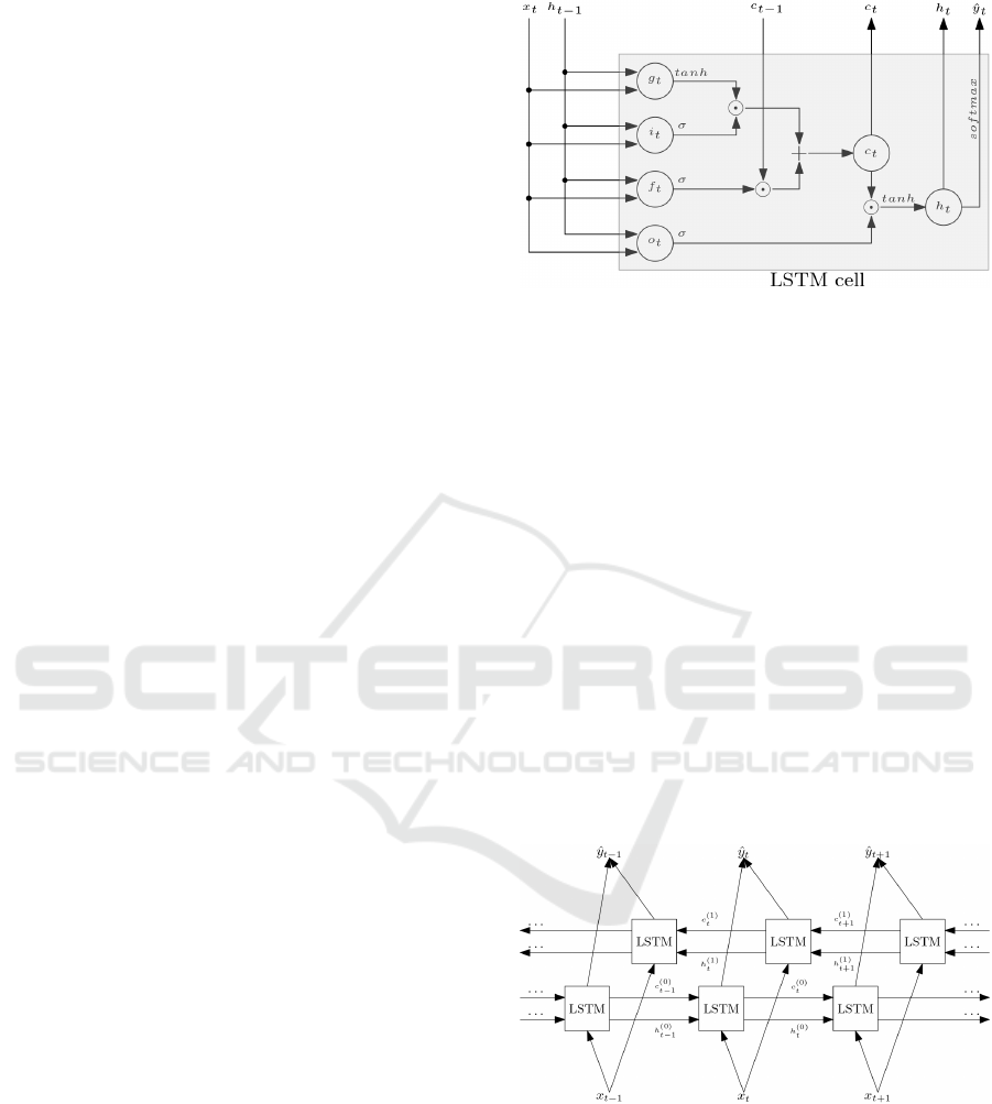
To see the detailed illustration of LSTM cell see
Figure 2.
Presented LSTM architecture in Figure 2 closely
maps the state-of-the-art design from (Zaremba et al.,
2014). Note that we dropped the network’s parame-
ters, matrices of weights, and vectors of biases to keep
it well-arranged.
Figure 2: Example of the LSTM architecture.
3.2.1 Bidirectional Long Short-term Memory
The traditional LSTM networks, the same as standard
recurrent neural networks and bidirectional recurrent
neural networks (BRNNs), are not suitable for some
tasks as the hidden and cell states are determined only
by prior states. Such tasks include text and speech re-
cognition and many more where the output at a time t
depends on the past as well as future inputs or labeling
problems where the output is only expected after fin-
ishing the whole input sequence (Graves, 2012). Bi-
directional Long Short-Term Memory or shortly
(BLSTM) networks try to solve this problem by hav-
ing connections both from the past and future cells.
Input to the BLSTM network is then presented in two
rounds, once forwards as with the LSTM network and
then in a reversed direction from the back. This archi-
tecture was introduced in (Graves and Schmidhuber,
2005).
Figure 3: Structure of BLSTM network.
In Figure 3 we can see the structure of BLSTM
network, the (0) and (1) in superscripts stand for for-
wards and backwards directions, respectively. We
omitted the detailed representation of LSTM cells to
make the illustration simpler.
BLSTM networks can be used to solve similar
problems as bidirectional RNNs where we have entire
input available beforehand. Training the network in
ICISSP 2021 - 7th International Conference on Information Systems Security and Privacy
518

forward and backward directions helps to gain context
from the past and future as well (Brownlee, 2019). In
addition, having hidden and cell state enables better
storage of information across the timeline even from
the distant past or future.
BLSTM networks were found to outperform
standard BRNNs in many tasks, e.g. speech recog-
nition. This was proven in the first application of
BLSTM networks by Graves et al. for phoneme clas-
sification problem (Graves and Schmidhuber, 2005).
BLSTMs are not suitable for all tasks, such as where
we do not know the final length of the input, and
the results are required after each timestamp (online
tasks).
3.3 Autoencoder
Autoencoder is a type of neural network that can
learn a representation of given data by compressing
and decompressing the input values. As described in
(Chollet, 2016), it consists of two parts, the encoder
and decoder. The encoder is typically a dense feed-
forward neural network (other types of neural net-
works can be used as well) with subsequent layers
shrinking in width. The decoder mirrors the struc-
ture of the encoder with expanding layers. The au-
toencoder is then trained with a set of data where in-
put matches the target output. After training, the de-
coder is detached and the encoder is used as the sole
model for prediction. The illustration of the autoen-
coder setup can be seen in Figure 4.
Figure 4: Example of autoencoder for digit compression
(Chollet, 2016).
Although the data compressed by autoencoder
could be used in image compression, generally au-
toencoders do not outperform well-known compres-
sion algorithms. Since the compression inside autoen-
coders is not lossless (the output is fuzzy), they are not
suitable for practical use of image compression.
Among places where autoencoders found utiliza-
tion belong dimension reduction and data denoising
problems. In dimension reduction, autoencoders are
used either as a preprocessing stage in machine learn-
ing problems or before data visualization where large
data dimension hinders the comprehension of the im-
age. In data denoising, the autoencoder is trained with
noisy images as the input and clear pictures being the
output. The use of autoencoders is not limited to im-
ages, however, they can also be used with audio and
other problems affected by noisiness.
4 FEATURE
TRANSFORMATIONS USING
LSTM NETWORKS
In this section, we present our approach - feature
transformation using LSTM networks. We describe
feature extraction and preparation, then feature selec-
tion along with the central part of this paper, the fea-
ture transformation using LSTM networks. Our com-
plete workflow is illustrated in Figure 8 at the end of
this section.
4.1 Feature Extraction
For extracting features from PE files, we used Py-
thon module pefile (Carrera, 2017). This module
extracts all PE file attributes into an object from which
they can be easily accessed. The structure of the PE
files is briefly explained in Section 3.1. We used as
many PE attributes as possible and reached the total
number of 303 features. Features can be divided into
multiple categories based on their origin from the PE
file. A summary of all target static features used in
our experiments is as follows:
Headers: Data from DOS, NT, File, and Optional
headers.
Data Directories: Names and sizes of all data dir-
ectories. Also adding detailed information from
prevalent directories for instance IMPORT, EX-
PORT, RESOURCE, and DEBUG directories.
Sections: Names, sizes, entropies of all PE sections
expressed by their average, min, max, mean and
standard deviation. To cooperate with a variable
amount of sections in different files, we decided
to describe only the first four and last sections in-
dividually.
Others: Extra characteristics associated with a file,
e.g. byte histogram, printable strings, or version
information.
4.2 Feature Preparation
Since not all machine learning models used in our
experiments can handle strings and other categorical
data, we must such data types encode into numeric
values. This strategy is necessary for more than 60
out of 303 columns. We chose to perform common
Representation of PE Files using LSTM Networks
519

transformation techniques on the entire dataset as op-
posed to only using the training set. We believe that
by doing so, we can better focus on designing LSTM
architectures and our results won’t be affected by the
capability of other algorithms.
4.2.1 Vectorization
Upfront, we transformed string features into sparse
matrix representation using TfidfVectorizer from
the scikit-learn Python library (Pedregosa et al.,
2011). This class demands corpus (collection of doc-
uments) as an input. We also adjusted parameters
stop_words and max_df that influence which words
to exclude from further calculations. Among the ex-
cluded words are either commonly used words in a
given language, words that do not bear any mean-
ing, and words that occur with such high frequencies
that they are not statistically interesting for us. To
eliminate the massive rise of dimensionality, we set
max_features parameter according to the feature’s
cardinality. The transformation itself consists of con-
verting sentences to vectors of token counts. Then
they are transformed into tf-idf representation. Tf-idf
is an abbreviation for the term frequency times inverse
document frequency. It is a way to express the weight
of a single word in the corpus (Maklin, 2019).
Term Frequency is the frequency of a word inside
the document. The formula is:
tf(w, d) =
n
w,d
∑
k
n
k,d
, (8)
where n
w,d
is the number of times word w appears
in a document d and the denominator is the sum of all
words found in d.
Inverse Document Frequency is a scale of how
much a word is rare across the whole corpus:
idf(w, D) = log
|D|
|d ∈ D : w ∈ d|
(9)
It is a fraction of the total number of documents
in corpus D divided by the number of documents con-
taining the specific word.
Tf-idf is then calculated as a multiplication of
these two values as follows:
tf-idf(w, d) = tf(w, d) · idf(w, D) (10)
All of this is done by the aforementioned class
TfidfVectorizer, and as a result, we get a matrix
of tf-idf features that can be used in further computa-
tions.
4.2.2 Hashing
For non-string values, we used a technique called fea-
ture hashing. This approach turns the column of
values into a sparse matrix using the value’s hash
as an index to the matrix. For this task, we used
FeatureHasher also from the scikit-learn. The
class takes an optional argument n_features which
limits the number of columns in the output matrix. We
set this argument dynamically according to the size of
the feature’s value set.
4.3 Feature Selection
Even though we tried to limit the rise of new features,
we ended up with 1488 features. To speed up the
forthcoming training process, we tried several feature
selection techniques to reduce the dimensionality of
the dataset.
Before all else, we filled missing values by
column’s mean and divided data into train and test
splits to ensure correct evaluation of the model’s per-
formance. For this, we used train_test_split
from sklearn.model_selection with test split
taking 20% of the dataset. Afterwards, we
transformed features to stretch across a smaller
range. For this task, we looked for another class
from sklearn.preprocessing library and selected
MinMaxScaler. This scaler turns each feature x to lie
between zero and one. The transformation is calcu-
lated as:
x
i
− min(x)
max(x) − min(x)
(11)
For feature selection, we settled with PCA (Prin-
cipal Component Analysis) with the number of com-
ponents determined by testing conducted with the
state-of-the-art ML algorithms: AdaBoost, Decision
tree, Feed-forward neural network, Random forest,
K-nearest neighbours, Support vector machine, Gaus-
sian naive bayes, and Logistic regression. The same
ML algorithms were used to evaluate performance of
LSTM-based transformation (see Section 5.2). We
tested a number of components ranging from 2 to
1400, however increasing benefits were found only
until 50 components, after which we did not measure
any significant improvements. The results are presen-
ted in Figure 5.
Note that while the resulting components are not
primarily in the form of sequences, they can still be
sequentially processed using the LSTM and achieve
solid classification results (see Section 5.3).
ICISSP 2021 - 7th International Conference on Information Systems Security and Privacy
520
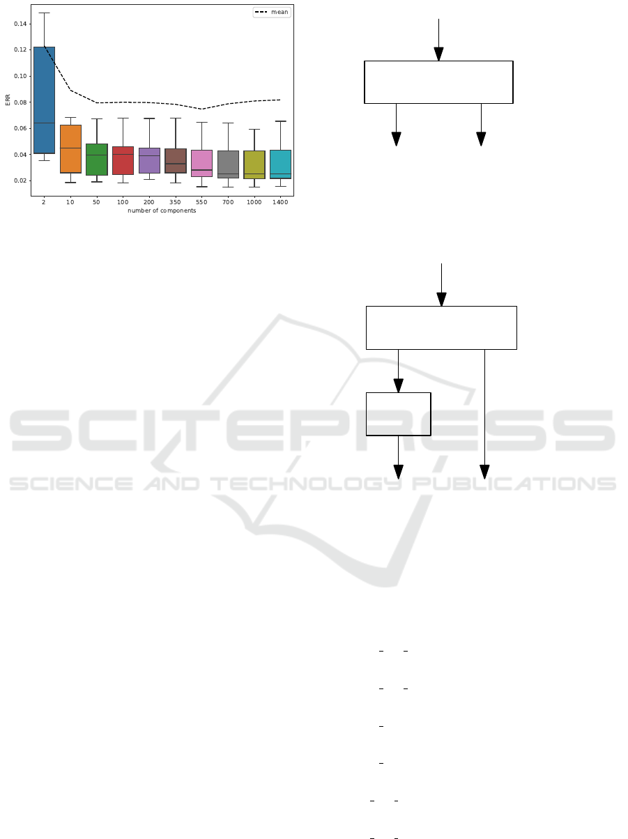
Figure 5: Average error rate (ERR) of ML algorithms across
number of components.
4.4 Feature Transformation using
LSTM Network
We experimented with various LSTM architectures
which we used for feature transformation. All net-
works were trained only on the train set. After the
training process, the train and test set were trans-
formed using the LSTM network.
Our research is not limited to only LSTM net-
works, however, bidirectional version of LSTM net-
works (BLSTM) was also included in our exper-
iments. We considered two different types of
neural networks: the Basic version consisting of
one (B)LSTM layer and the Deep version with four
(B)LSTM layers, each layer containing 50 LSTM
units equal to the number of input features. All net-
works were trained up to 50 epochs with a batch size
of 32, Adam optimization, and mean squared error
loss function.
4.4.1 Type 1
The first type of LSTM network we experimented is
based on autoencoder’s architecture. In this case, we
worked only with explanatory variables with a net-
work designed to predict the same values which were
given on input. The predicted transformation was
taken from the penultimate layer’s last hidden state.
Schema of the Type 1 transformer is illustrated in Fig-
ure 6.
4.4.2 Type 2
The second type was similar to the regular use of the
LSTM network, where we work with both the explan-
atory and response variables. For prediction, we used
the last hidden state of the penultimate LSTM layer as
with Type 1. The last layer was occupied by a single
(B)LSTM layer
y
Output
Predicted
transformation
h
t
X
Input
Figure 6: Schema of Basic version Type 1 transformer.
neuron with a sigmoid activation function. Diagram
of the Type 2 transformer is presented in Figure 7.
(B)LSTM layer
y
Input
Output
Predicted
h
t
X
Dense
layer
transformation
Figure 7: Schema of Basic version Type 2 transformer.
4.4.3 Description of All Transformed Datasets
The following is a description of the datasets used in
testing. Recall that ”Basic” and ”Deep” in the de-
scription below denote one layer and four layers of
the deep network, respectively:
BLSTM AE basic Transformed by Basic version of
BLSTM Type 1 (autoencoder) network.
BLSTM AE deep Transformed by Deep version of
BLSTM Type 1 (autoencoder) network.
BLSTM basic Transformed by Basic version of
BLSTM Type 2 network.
BLSTM deep Transformed by Deep version of
BLSTM Type 2 network.
LSTM AE basic Transformed by Basic version of
LSTM Type 1 (autoencoder) network.
LSTM AE deep Transformed by Deep version of
LSTM Type 1 (autoencoder) network.
Representation of PE Files using LSTM Networks
521
LSTM basic Transformed by Basic version of
LSTM Type 2 network.
LSTM deep Transformed by Deep version of LSTM
Type 2 network.
VANILLA Control dataset, no transformations
made.
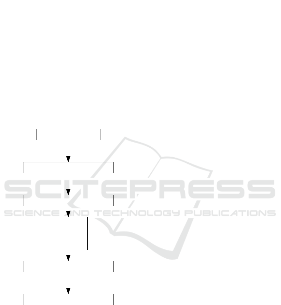
4.5 Evaluation using Supervised ML
Algorithms
The final part of the experiment workflow consists
of evaluation of the aforementioned transformations.
We tested several supervised ML algorithms and com-
pared their performance on vanilla and transformed
datasets. Detailed description of this part can be
found in Section 5.2. Figure 8 overviews the exper-
iment pipeline.
PE files
Static features
Vanilla Dataset
(B)LSTM
network
Transformed Dataset
Results
ML algorithms
Feature selection
(PCA)
Feature preparation
Feature extraction
Figure 8: Experiment pipeline.
5 EXPERIMENTS
In this section, we firstly describe the dataset used in
our experiments. Then we specify our experimental
setup in detail and evaluation methods, and in the end,
we present our results.
5.1 Dataset
We gathered a dataset of 30,154 samples which
are evenly distributed between malware and be-
nign files. For amassing benign files, we searched
disks on university computers and the malware files
were obtained from an online repository https://
virusshare.com which we thanks for the access.
5.2 Experimental Setup and Evaluation
Methods
The performance of LSTM pre-treatment was eva-
luated by the following supervised ML algorithms.
Among the ML algorithms we used were Support
vector classification (SVC) with kernel rbf, deep
Feed-forward network (FNN) with 8 hidden layers
(128-128-64-64-32-32-16-16 neurons per layer) all
with ReLU activation function, trained up to 200
epochs with Adam optimization and binary cross-
entropy loss function. Further, we tested Decision
tree, Random forest, AdaBoost, K-nearest neighbours
(k=5), Gaussian naive bayes, and Logistic regres-
sion. The hyperparameters which we did not men-
tion were left to default settings as set by authors of
the scikit-learn library (Pedregosa et al., 2011) ex-
cept for the FNN which was modeled with the help of
the Python deep learning library Keras (Chollet et al.,
2015).
Our implementation was executed on a single
computer platform having two processors (Intel Xeon
Gold 6136, 3.0GHz, 12 cores each), with 32 GB of
RAM running the Ubuntu server 18.04 LTS operating
system.
5.2.1 Metrics
In this section, we present the metrics we used to
measure the performance of our proposed classific-
ation models. For evaluation purposes, the following
classical quantities are employed:
True Positive (TP) represents the number of mali-
cious samples classified as malware.
True Negative (TN) represents the number of benign
samples classified as benign.
False Positive (FP) represents the number of benign
samples classified as malware
False Negative (FN) represents the number of mali-
cious samples classified as benign.
The performance of our classifiers on the test set
is measured using the following standard metrics:
ICISSP 2021 - 7th International Conference on Information Systems Security and Privacy
522
Accuracy (ACC) Proportion of correctly classified
samples out of all predictions:
ACC =
T P + T N
T P + T N + FP + FN
(12)
Error rate (ERR) The inverse of accuracy:
ERR = 1 − ACC (13)
Sensitivity (TPR, Recall) How many samples from
the positive class were predicted correctly:
T PR =
T P
T P + FN
(14)
Fall-out (FPR) Probability of predicting samples
from the negative class as positives:
FPR =
FP
FP + T N
(15)
5.3 Results
In order to expose any biases in the data, we tested
the ML algorithms with 5-fold cross-validation using
cross_validate from scikit-learn library.
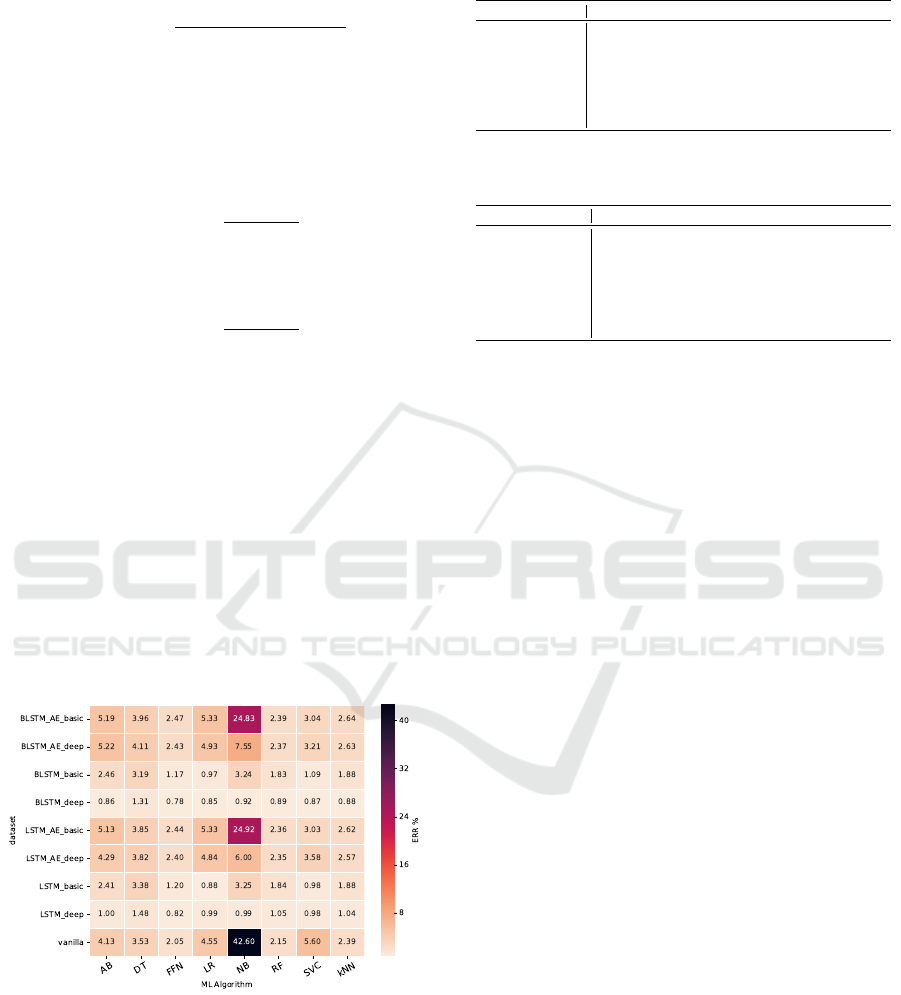
We found that the results did not only vary
between different network architectures but also
among particular ML algorithms. These observations
are presented in the heatmap in Figure 9. These res-
ults indicate that Type 1 based on autoencoder design
does not seem to improve the performance whatso-
ever. However, Type 2, especially deep versions of
LSTM and BLSTM networks, seem to enhance the
performance of many algorithms significantly.
Figure 9: Heatmap comparing the ERR of ML algorithms
with respect to different transformer architectures.
Tables 1, 2 and 3 present the improvements made
by pre-treatment with LSTM and BLSTM networks
for different ML algorithms used for evaluation. Note
that the performance of Logistic regression, Naive
Bayes, SVC, or AdaBoost algorithms increased the
most significantly.
Table 1: Baseline results of ML algorithms on unedited
(vanilla) dataset.
ML Algorithm ACC TPR FPR ROC-AUC
AdaBoost 95.87 ± 0.39 95.49 ± 0.55 3.75 ± 0.46 95.87 ± 0.39
DecisionTree 96.47 ± 0.20 96.37 ± 0.25 3.44 ± 0.40 96.47 ± 0.20
Feed-ForwardNetwork 97.95 ± 0.12 97.75 ± 0.36 1.86 ± 0.23 97.95 ± 0.12
LogisticRegression 95.45 ± 0.38 94.62 ± 0.38 3.73 ± 0.45 95.45 ± 0.38
NaiveBayesGaussian 57.40 ± 16.01 16.63 ± 36.13 1.84 ± 4.11 57.40 ± 16.01
RandomForest 97.85 ± 0.20 97.52 ± 0.24 1.82 ± 0.19 97.85 ± 0.20
SVC(kernel=rbf) 94.40 ± 1.74 93.49 ± 1.74 4.69 ± 1.81 94.40 ± 1.74
kNN(k=5) 97.61 ± 0.21 97.17 ± 0.28 1.94 ± 0.16 97.61 ± 0.21
Table 2: Results of ML algorithms on dataset transformed
by deep LSTM network.
ML Algorithm ACC TPR FPR ROC-AUC
AdaBoost 99.00 ± 0.71 98.76 ± 0.78 0.76 ± 0.66 99.00 ± 0.71
DecisionTree 98.52 ± 0.55 98.43 ± 0.60 1.40 ± 0.50 98.52 ± 0.55
Feed-ForwardNetwork 99.18 ± 0.77 99.10 ± 0.64 0.75 ± 0.90 99.18 ± 0.77
LogisticRegression 99.01 ± 0.72 98.89 ± 0.78 0.87 ± 0.67 99.01 ± 0.72
NaiveBayesGaussian 99.01 ± 0.67 98.70 ± 0.58 0.69 ± 0.78 99.01 ± 0.67
RandomForest 98.95 ± 0.77 98.85 ± 0.77 0.95 ± 0.78 98.95 ± 0.77
SVC(kernel=rbf) 99.02 ± 0.72 98.73 ± 0.74 0.69 ± 0.70 99.02 ± 0.72
kNN(k=5) 98.96 ± 0.75 98.82 ± 0.80 0.91 ± 0.71 98.96 ± 0.75
The performance of the two most successful clas-
sifiers evaluated on all transformed datasets con-
sidered in our experiments, Feed-forward neural net-
work, and Logistic regression, is presented in Figure
10.
To emphasize our results, we express the perform-
ance of the ML algorithms in terms of error rate (in
[%]). In Table 4, we overview the error rates (ERR)
of ML algorithms evaluated on the original and trans-
formed dataset by deep BLSTM network.
6 CONCLUSIONS
We collected a large number of PE binaries from
available resources. From these binaries, we extrac-
ted as many features as possible, which we later scale
down by the feature selection algorithm PCA in order
to reduce the dimension of our dataset. After that, we
conducted extensive testing with various (B)LSTM
network architectures used to transform the selec-
ted features. On these transformed datasets, we ran
a cross-validation benchmark using multiple super-
vised ML algorithms to see whether the feature trans-
formation based on (B)LSTM networks can increase
the performance of the ML algorithms in comparison
to the performance to the accuracy on the vanilla data-
set.
We have found that the feature transformation by
(B)LSTM nets was hugely successful, decreasing er-
ror rate from 58.6% to 97.84% depending on the ML
algorithm used. These gains were achieved by so-
called Type 2 architecture which was similar to the
standard use of recurrent neural networks for clas-
sification problems. In contrast, the Type 1 design
based on autoencoder structure didn’t prove to en-
Representation of PE Files using LSTM Networks
523
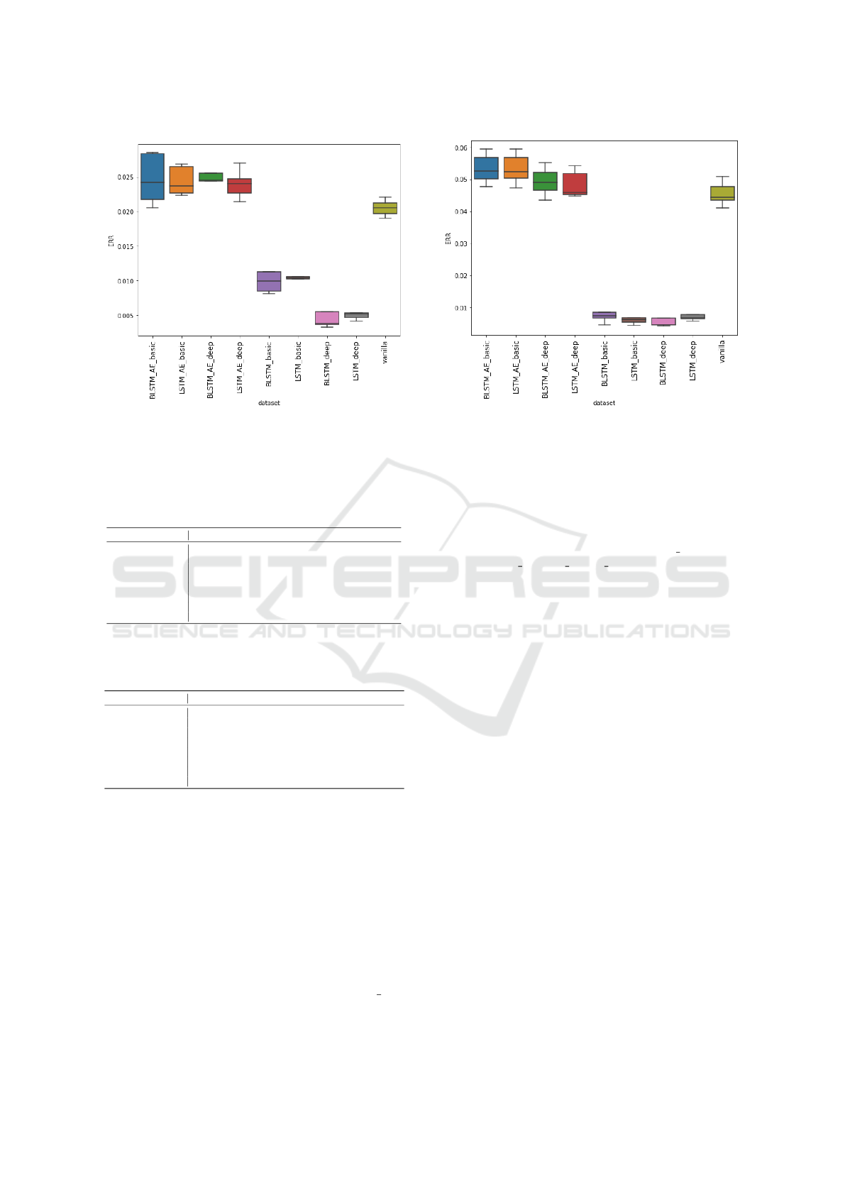
(a) Feed-forward neural network. (b) Logistic regression.
Figure 10: Boxplots showing the performance of the two most successfull classifiers evaluated on multiple datasets.
Table 3: Results of ML algorithms on dataset transformed
by deep BLSTM network.
ML Algorithm ACC TPR FPR ROC-AUC
AdaBoost 99.14 ± 0.77 99.06 ± 0.81 0.78 ± 0.80 99.14 ± 0.77
DecisionTree 98.69 ± 0.71 98.67 ± 0.79 1.30 ± 0.65 98.69 ± 0.71
Feed-ForwardNetwork 99.22 ± 0.84 99.12 ± 0.87 0.67 ± 0.83 99.22 ± 0.84
LogisticRegression 99.15 ± 0.78 99.07 ± 0.81 0.78 ± 0.79 99.15 ± 0.78
NaiveBayesGaussian 99.08 ± 0.78 98.65 ± 0.82 0.48 ± 0.77 99.08 ± 0.78
RandomForest 99.11 ± 0.74 99.01 ± 0.80 0.78 ± 0.72 99.11 ± 0.74
SVC(kernel=rbf) 99.13 ± 0.82 98.94 ± 0.87 0.67 ± 0.79 99.13 ± 0.82
kNN(k=5) 99.12 ± 0.82 99.02 ± 0.87 0.78 ± 0.79 99.12 ± 0.82
Table 4: Comparison of the results achieved from the ML
algorithms evaluated on the vanilla (non-transformed) data-
set and the transformed dataset by deep BLSTM network.
ML Algorithm ERR (no LSTM) ERR (with LSTM) ERR decreased by
AdaBoost 4.13 0.86 79.18
DecisionTree 3.53 1.31 62.89
Feed-ForwardNetwork 2.05 0.78 61.95
LogisticRegression 4.55 0.85 81.32
NaiveBayesGaussian 42.60 0.92 97.84
RandomForest 2.15 0.89 58.60
SVC(kernel=rbf) 5.60 0.87 84.46
kNN(k=5) 2.39 0.88 63.18
hance performance. The transformation by Type 2
deep transformers brought all tested ML algorithms
to a similar level. The smaller performance in-
crements were observed among the ML algorithms
which already performed well on the non-transformed
dataset.
ACKNOWLEDGEMENTS
The authors acknowledge the support of the OP VVV
MEYS funded project CZ.02.1.01/0.0/0.0/16 019/
0000765 ”Research Center for Informatics”.
REFERENCES
AV-test (2019). Security report 2018/19. https:
//www.av-test.org/fileadmin/pdf/security report/
AV-TEST Security Report 2018-2019.pdf.
Barron, D. W. (1978). Assemblers and loaders. Elsevier
Science Inc.
Brownlee, J. (2019). How to develop a bidirectional
lstm for sequence classification in python with
keras. https://machinelearningmastery.com/develop-
bidirectional-lstm-sequence-classification-python-
keras/.
Carrera, E. (2017). Pefile. https://github.com/erocarrera/
pefile.
Chollet, F. (2016). Building autoencoders in keras. https:
//blog.keras.io/building-autoencoders-in-keras.html.
Chollet, F. et al. (2015). Keras. https://keras.io.
Graves, A. (2012). Supervised sequence labelling. In Su-
pervised sequence labelling with recurrent neural net-
works, pages 13–39. Springer.
Graves, A. and Schmidhuber, J. (2005). Framewise phon-
eme classification with bidirectional lstm and other
neural network architectures. Neural networks, 18(5-
6):602–610.
Hardy, W., Chen, L., Hou, S., Ye, Y., and Li, X. (2016).
Dl4md: A deep learning framework for intelligent
malware detection. In Proceedings of the Interna-
tional Conference on Data Mining (DMIN), page 61.
The Steering Committee of The World Congress in
Computer Science, Computer . . . .
Hochreiter, S. and Schmidhuber, J. (1997). Long short-term
memory. Neural computation, 9(8):1735–1780.
Karl Bridge, M. (2019). Pe format - win32 apps.
”https://docs.microsoft.com/en-us/windows/win32/
debug/pe-format”.
ICISSP 2021 - 7th International Conference on Information Systems Security and Privacy
524

Kowalczyk, K. (2018). Portable executable file
format. https://blog.kowalczyk.info/articles/
pefileformat.html.
Latto, N. (2020). What is wannacry? https://
www.avast.com/c-wannacry.
Leskovec, J., Rajaraman, A., and Ullman, J. D. (2020). Min-
ing of massive data sets. Cambridge university press.
Lipton, Z. C., Berkowitz, J., and Elkan, C. (2015). A crit-
ical review of recurrent neural networks for sequence
learning. arXiv preprint arXiv:1506.00019, pages 5–
25.
Lu, R. (2019). Malware detection with lstm using opcode
language. arXiv preprint arXiv:1906.04593.
Maklin, C. (2019). Tf idf: Tfidf python example.
https://towardsdatascience.com/natural-language-
processing-feature-engineering-using-tf-idf-
e8b9d00e7e76.
Pedregosa, F., Varoquaux, G., Gramfort, A., Michel, V.,
Thirion, B., Grisel, O., Blondel, M., Prettenhofer,
P., Weiss, R., Dubourg, V., Vanderplas, J., Passos,
A., Cournapeau, D., Brucher, M., Perrot, M., and
Duchesnay, E. (2011). Scikit-learn: Machine learning
in Python. Journal of Machine Learning Research,
12:2825–2830.
Saxe, J. and Berlin, K. (2015). Deep neural network based
malware detection using two dimensional binary pro-
gram features. In 2015 10th International Conference
on Malicious and Unwanted Software (MALWARE),
pages 11–20. IEEE.
Symantec, C. (2019). Internet security threat report 2019.
https://docs.broadcom.com/doc/istr-24-2019-en.
Vinayakumar, R., Soman, K., Poornachandran, P., and
Sachin Kumar, S. (2018). Detecting android malware
using long short-term memory (lstm). Journal of In-
telligent & Fuzzy Systems, 34(3):1277–1288.
Zaremba, W., Sutskever, I., and Vinyals, O. (2014). Re-
current neural network regularization. arXiv preprint
arXiv:1409.2329, pages 1–3.
Zhou, H. (2018). Malware detection with neural network
using combined features. In China Cyber Security An-
nual Conference, pages 96–106. Springer.
Representation of PE Files using LSTM Networks
525
