
Extending StructureNet to Generate Physically Feasible 3D Shapes
Jannik Koch
1,2
, Laura Harak
´
e
1
, Alisa Jung
2
and Carsten Dachsbacher
2
1
Fraunhofer Institute of Optronics, System Technologies and Image Exploitation IOSB, Ettlingen, Germany
2
Karlsruhe Institute of Technology, Karlsruhe, Germany
Keywords:
Generative Models, Shape Synthesis, Graph Neural Networks, Physical Constraints, Measure of Infeasibility.
Abstract:
StructureNet is a recently introduced n-ary graph network that generates 3D structures with awareness of
geometric part relationships and promotes reasonable interactions between shape parts. However, depending
on the inferred latent space, the generated objects may lack physical feasibility, since parts might be detached
or not arranged in a load-bearing manner. We extend StructureNet’s training method to optimize the physical
feasibility of these shapes by adapting its loss function to measure the structural intactness. Two new changes
are hereby introduced and applied on disjunctive shape parts: First, for the physical feasibility of linked parts,
forces acting between them are determined. Considering static equilibrium, compression and friction, they are
assembled in a constraint system as the Measure of Infeasibility. The required interfaces between these parts
are identified using Constructive Solid Geometry. Secondly, we define a novel metric called Hover Penalty that
detects and penalizes unconnected shape parts to improve the overall feasibility. The extended StructureNet
is trained on PartNet’s chair data set, using a bounding box representation for the geometry. We demonstrate
first results that indicate a significant reduction of hovering shape parts and a promising correction of shapes
that would be physically infeasible.
1 INTRODUCTION
Tools that automate the generation of 3D shapes are
an important aid for creators of entertainment media,
like video games or film, and researchers using physi-
cal simulations. Due to this demand, various procedu-
ral modeling techniques trying to provide results that
are both diverse and available in vast quantities have
been proposed before.
Early grammar-based methods are able to produce
a large variety of shapes by relying on sets of gen-
erative descriptions. While these usually work well
for simple shapes, the underlying rules become more
complex or even contradictory the more detailed the
shapes to be generated are. The difficulty of describ-
ing the detailed makeup of complex shapes as gram-
mars encouraged alternative methods that infer the
synthesis rules from exemplary data.
In the context of shape analysis and (part-based)
shape synthesis, advanced methods like (Ma et al.,
2014) capture geometric properties for mapping an
exemplary source model to a target model at various
levels of complexity. More generally, inferring com-
plex behavior from data is a core component in the
field of artificial neural networks.
Recent generative models leverage Variational
Autoencoders (VAEs) or Generative Adversarial Net-
works (GANs) to create 3D shapes without using
heuristics for detecting the underlying object struc-
ture, but rather learning it (Goodfellow et al., 2016).
The StructureNet (Mo et al., 2019a) framework used
in this paper not only considers the geometry, but also
the part relationships in the learning process by rep-
resenting shapes as hierarchical graphs. This allows
for the generation of shapes of novel structure and ge-
ometry, as well as editing shapes or shape parts while
preserving the structural hierarchy.
While the generated objects mostly maintain a vi-
sual plausibility, the assembled latent space the new
shapes are drawn from may still hold non-functional
or defective shapes with asymmetrical or missing
parts. Physically correct interactions with such shapes
are often impractical. A possible reason for the gener-
ation of defective shapes is an underrepresentation of
the respective shape family in the training data. Since
gathering additional data is not always possible, this
paper aims to extend the training to explicitely pro-
mote physically feasible shapes in the training.
Our approach views the task as an inverse statics
problem. We provide two additional metrics in Struc-
tureNet’s training: For detached parts we present a
novel metric called the Hover Penalty that promotes
Koch, J., Haraké, L., Jung, A. and Dachsbacher, C.
Extending StructureNet to Generate Physically Feasible 3D Shapes.
DOI: 10.5220/0010256702210228
In Proceedings of the 16th International Joint Conference on Computer Vision, Imaging and Computer Graphics Theory and Applications (VISIGRAPP 2021) - Volume 1: GRAPP, pages
221-228
ISBN: 978-989-758-488-6
Copyright
c
2021 by SCITEPRESS – Science and Technology Publications, Lda. All rights reserved
221
parts being in contact with each other. Furthermore
we apply a linear constraint system to calculate the
Measure of Infeasibility introduced by (Whiting et al.,
2009) to evaluate the overall physical feasibility.
2 RELATED WORK
Generative Models: Various attempts at generating
3D geometry by inferring a generative model have
been made prior to StructureNet (Mo et al., 2019a).
(Kalogerakis et al., 2012) train a probabilistic
model on a set of compatibly segmented shapes.
The VAE (Kingma and Welling, 2013) used by
StructureNet is a common approach to achieve this
goal. 3D-GAN (Wu et al., 2016) uses Generative
Adversarial Networks (GANs) and achieves results
of similar quality. While both architectures generate
novel shapes that successfully imitate the original
input, neither implementation currently considers
physical limitations. This paper attempts to mitigate
that.
Static Analysis: Since StructureNet uses an
approach based on neural networks, we achieve the
consideration of physical feasibility by extending the
total loss for which the network adjusts its weights.
These new components of the loss function are
based on previous research about physical feasibility.
(Whiting et al., 2009) present an approach to optimize
masonry shapes, like cathedrals or unreinforced con-
crete dams, for physical feasibility. While focusing
on buildings, their approach works well with arbitrary
3D geometry and provides the means for automatic
adjustments of massive shapes.
Further research in the field of structural sound-
ness focuses on 3D printing. For example, (Pr
´
evost
et al., 2013) tackle balancing a 3D shape before
printing. Furthermore, (Stava et al., 2012) optimize
3D printable shapes for physical feasibility and
additionally try to maximize robustness for subse-
quent cleaning and transportation. While providing
impressive results, both optimization approaches
hollow out shapes, which does not translate well to
our use case as we want to focus on massive shapes
that are often found in real life. This makes the
approach by (Whiting et al., 2009) the more sensible
choice. Additionally, the findings by (Pr
´
evost et al.,
2013) focus on a solution that assists a human
designer. Since the findings by (Whiting et al., 2009)
tune shapes in a fully automatic fashion, they lend
themselves more to a machine learning approach as
employed by us.
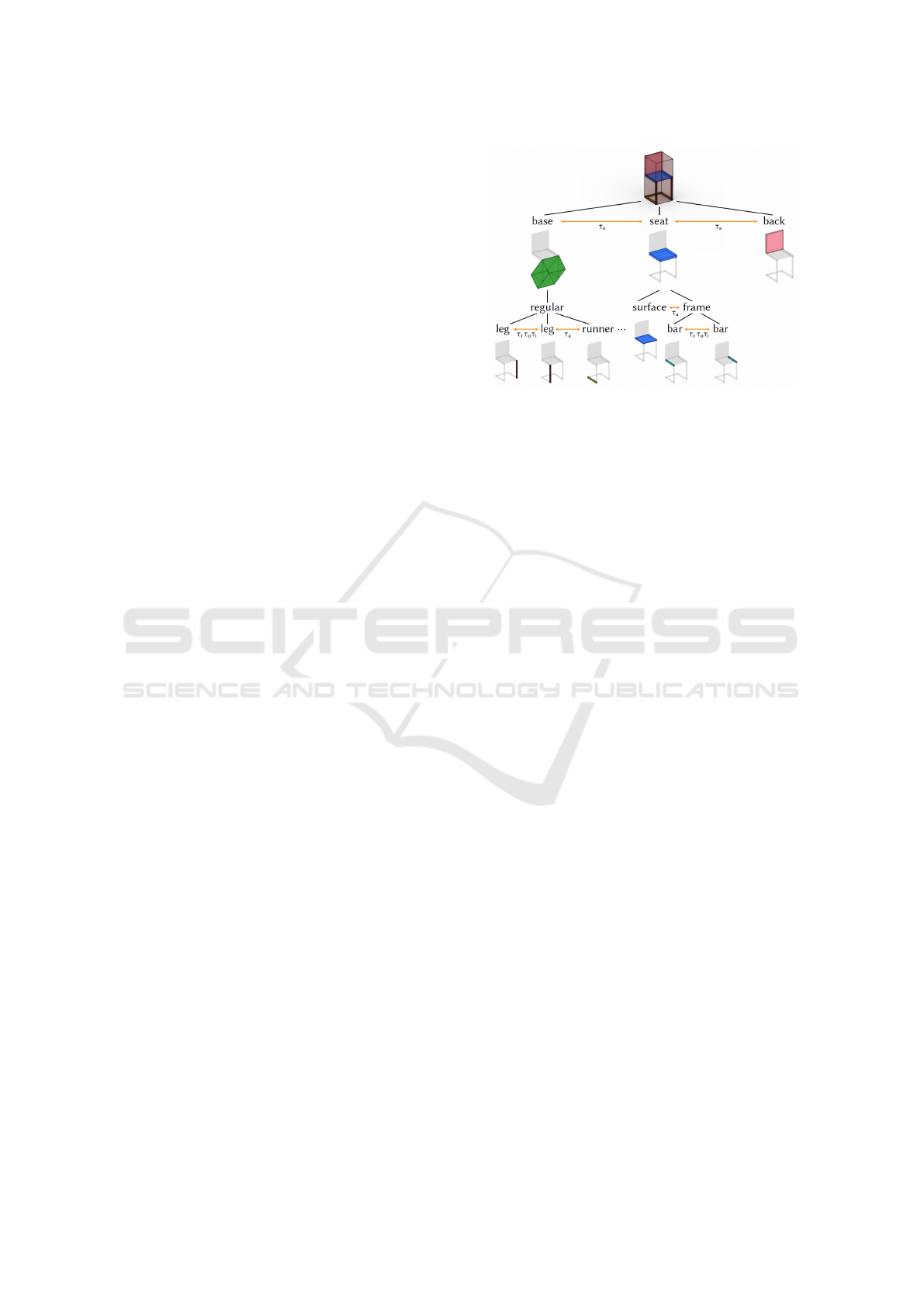
Figure 1: The representation of a chair from the Part-
Net (Mo et al., 2019b) data set as an n-ary graph created
by (Mo et al., 2019a). The shape parts are hierarchically or-
dered (black edges), geometrically represented as oriented
bounding boxes and semantically labeled accordingly (col-
ors). The orange horizontal edges describe geometric re-
lationships between parts, specifically adjacency (τ
a
) and
translational, reflective or rotational symmetries (τ
t
, τ
r
, τ
o
).
Constructive Solid Geometry: In order to eval-
uate the physical feasibility of a shape we need to
compute the contact surfaces between the shape’s
parts. We achieve this by employing intersection op-
erations provided through Constructive Solid Geome-
try (CSG) (Laidlaw et al., 1986) on the part geometry.
The choice of CSG is due to the fact that it works on
arbitrary geometry and computes a geometrical repre-
sentation of the interactions.
3 STRUCTURENET
FRAMEWORK
StructureNet is a graph neural network that generates
multi-part 3D models (shapes) with varying structure
and geometry. Its essential component is an n-ary
graph that represents the overall structure of a shape
and thus allows to organize its parts hierarchically
as nodes. Additionally, geometric relationships like
adjacencies or symmetries between part siblings are
considered as horizontal edges within that graph as
shown in Figure 1.
StructureNet is a generative approach in the
context of both shape analysis and shape synthesis of
graph structured shape data. It is trained and tested
with the PartNet data set (Mo et al., 2019b) which
already classifies shapes into model categories and
contains hierarchically ordered and semantically
labeled shape part geometries. The geometry is either
represented as point clouds or oriented bounding
boxes and fed into a Variational Autoencoder (VAE).
GRAPP 2021 - 16th International Conference on Computer Graphics Theory and Applications
222

Figure 2: Examples of incorrectly generated chairs by the
original StructureNet (Mo et al., 2019a): Hovering parts
(left), asymmetrical shape parts (middle) or overlapping
shape parts (right) are addressed by the Measure of Infeasi-
bility and Hover Penalty introduced in this paper.
The VAE consists of two hierarchical graph networks
that convolve a shape’s graph. In the following para-
graphs we briefly recap StructureNet’s architecture
and training workflow.
Architecture: The VAE is composed of a group
of two encoders (e) and a group of two decoders (d)
that learn a mapping from a shape S to a feature vec-
tor z and the shape’s reconstruction S
0
from z with
S
0
= d(e(S)). Both groups trace the graph of S recur-
sively in a bottom-up (e) and top-down (d) order, each
encoder and decoder handling either the geometry of
a shape part (leaf node) itself or a child graph of a
part. Here, a geometry encoder induces a feature vec-
tor from the leaf nodes by processing the geometric
representation of the corresponding shape parts (point
clouds or bounding boxes) differently. A graph en-
coder then encodes these intermediate feature vectors
of each part and each part relationship recursively to
get z for the entire input shape S.
Starting with z as the latent code of the root node,
a graph decoder recursively transforms it into child
graphs, where each node (shape part) and its edges
to other nodes (geometric relationships) are assigned
a probability predicting their (non-)existence. Nodes
and edges that are not predicted to exist are discarded,
existing nodes are decoded into their geometry rep-
resentation using a geometry decoder. Additionally,
the semantic label of a part and a probability of it
being a leaf node for ending recursion are determined.
Training: StructureNet’s training stage only con-
siders shapes with a limited number of child parts.
Fine-grained shapes with a hierarchy containing an
exceeding number of child parts are refused. The total
loss for learning a reversible mapping of a shape S to
z is minimized using Mini-Batch Gradient Descent:
L
total
= E
S ∼ S
[L
r
(S) + L
sc
(S) + βL
v
(S)]. (1)
E
S ∼ S
is the expected value of the summed losses for
a shape S to be drawn from a distribution of a certain
shape category S, such as tables, chairs or cabinets.
L
r
(S) is the loss function for learning to reconstruct
the shape S
0
= d(e(S)) from the ground truth shape
S. The correspondence between both shapes’ parts is
determined by solving a linear assignment problem,
matching their parts separately for each child graph.
For the exact composition of this reconstruction loss
see (Mo et al., 2019a). L
sc
(S) is the loss function for
structure consistency between the reconstructed part
geometries and edges, which aims at making parts
structurally consistent with their relationships, where
a relationship between two parts should also hold for
their subtrees. βL
v
(S) is a weighted variational regu-
larization loss for handling the distribution density of
shapes in the inferred latent space.
The total loss L
total
is calculated as a forward
propagation function, where batches with a certain
number of shapes from one category are fed into the
network to obtain the loss of each batch by summing
up the individual losses of each shape after encoding
and decoding. Since StructureNet still might produce
failure cases (Figure 2), we extend its total loss to ac-
count for the physical feasibility for every batch in
Section 5.
4 PHYSICAL FEASIBILITY
Physical feasibility is defined as the ability of a shape
to support its own weight. (Whiting et al., 2009)
model this as a system of constraints based on the
forces acting between shape parts. Determining
whether a shape is physically feasible is therefore
a task of finding a set of forces that satisfy these
constraints.
Constraints: All forces act on the vertices of
the contact surfaces between parts (“interfaces”). A
shape is considered physically feasible if a set of
forces exists that negates the gravitational forces of
every part while each force points in a “plausible”
direction. The situation in which all contact forces
negate each other and all gravitational forces is
referred to as static equilibrium. A plausible di-
rection of a force lies in a cone around the surface
normal, which limits the directions due to friction.
Furthermore, forces need to provide compression,
meaning they need to point away from the interface
in order to model parts pushing each other away.
This compression constraint prevents the presence of
“tension forces” which point in the opposite direction
and act as glue holding physically infeasible shapes
together. Figure 3 shows an example of the tension
and compression forces.
Measure of Infeasibility: The constraint system
only provides binary answers to the question of
Extending StructureNet to Generate Physically Feasible 3D Shapes
223
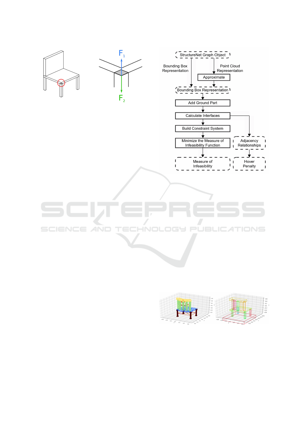
Figure 3: Visualization of the active forces at an exemplary
part interface. From the perspective of the chair leg, F
1
is
the tension force and F
2
the compression force. The di-
rection of the forces swaps when observing from the seat’s
perspective. In reality, only the compression force is needed
here as the seat presses down on the leg, satisfying the com-
pression constraint.
physical feasibility, since there either is or is not
a set of forces that satisfies the constraint system.
Therefore, (Whiting et al., 2009) soften the com-
pression constraint to allow for tension forces that
hold the shape together where necessary. Tension
forces are penalized, resulting in an optimization
problem where the squared sum of tension forces is
minimized. The minimum is the metric describing
the overall physical feasibility of the shape, called
the Measure of Infeasibility. The system of equations
describing the Measure of Infeasibility is shown in
Equation 2.
Extension: In order to extend StructureNet to ac-
count for physical feasibility, we include the Measure
of Infeasibility into the training stage. The new met-
ric serves as an additional element of the loss func-
tion and promotes the generation of physically feasi-
ble shapes. Our approach is comprised of the individ-
ual steps shown in Figure 4 and described further in
the following section.
5 EXTENSIONS
Graph Representation: The geometry generated by
StructureNet is arranged as a tree graph. In order to
assess the physical feasibility of a shape generated by
StructureNet, only the graph leaves are of concern as
they store the geometry of the individual parts. The
relationships between parts stored in the graph are
ignored: While adjacency relationships play a role in
later steps, they are not reliably provided in newly
generated data during training. Instead of relying
on the information stored in the graph, adjacency
relationships are therefore detected using intersection
checks during interface generation.
Figure 4: Visualization of the process by which the Measure
of Infeasibility and Hover Penalty is calculated from a graph
object.
Geometry Pre-processing: The original Struc-
tureNet implementation supports both point cloud and
bounding box representations, including semantic la-
bels. Instead of differentiating between these, we fo-
cus on the latter and support the former by approx-
imating point clouds with bounding boxes using the
findings by (Barequet and Har-peled, 2001). The re-
sults of the approximation are shown in Figure 5.
This avoids further case differentiations in subsequent
steps of our method. The tradeoff, however, is addi-
tional overhead and a loss of detail when using the
point cloud representation, which is discussed further
in Section 7. Last, we add a bounding box represent-
ing the ground to the overall geometry, so we can treat
the ground like any other shape part during interface
calculations.
Figure 5: Converting a point cloud shape into a bounding
box representation, including the addition of a ground part.
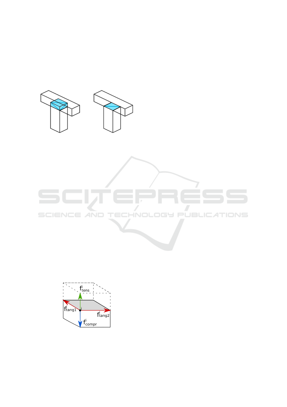
Interface Generation: We generate part inter-
faces using Boolean operations. Note that parts of
generated shapes not only share a polygonal contact
plane, but often intersect significantly. Therefore, in-
terfaces are deduced from the intersection volume.
GRAPP 2021 - 16th International Conference on Computer Graphics Theory and Applications
224
First, every possible pair of parts is checked for ad-
jacency by testing whether their Boolean intersection
volume is zero using CSG. If that is not the case, this
intersection volume is cut out from one of the two
parts chosen at random. The new triangles created by
this operation are then used as the interfaces between
the parts as shown in Figure 6.
Figure 6: Exemplary removal of an intersection volume,
yielding two new triangles used as part interfaces.
Hover Penalty: Since the Measure of Infeasibil-
ity requires a ground part to push back against the
shape for static equilibrium, it can only account for
parts with direct or indirect ground contact. We in-
troduce an additional penalty for parts or clusters of
parts hovering in mid-air. By keeping track of the
pairwise adjacencies found when calculating the in-
terfaces, we check parts for direct or indirect ground
contact. Direct contact with the ground is given if a
direct adjacency relationship with the ground part ex-
ists. Indirect contact with the ground is characterized
by a chain of adjacencies that lead to a part that is
in direct contact with the ground. For every part that
is not in direct or indirect contact with the ground, we
take the smallest possible Euclidean distance between
the centers of gravity to any part with direct or indirect
ground contact. The sum of these distances makes up
the additional Hover Penalty loss. The rationale be-
hind this is that parts should be nudged towards each
other until they can all be adjusted using the Measure
of Infeasibility.
Constraint System: Once the interfaces and the
Hover Penalty are calculated, the constraint system
Figure 7: Visualization of the force components that make
up any force acting on a vertex i. Note that the choice which
force is the compression force and which one is the tension
force is based on the perspective of the bottom part.
for the Measure of Infeasibility (Whiting et al., 2009)
shown in Equation 2 can be applied:
y(S) = min
f
∑
f
i
( f
i
tens
)
2
(2)
s.t. A
eq
· f + w = 0
A
f r
· f ≤ 0
A
compr
· f ≥ 0
with y being the Measure of Infeasibility of a shape
S. f is the concatenation of every force vector f
i
placed on an interface vertex i in the shape. Each
of these force vectors is further subdivided into four
components with respect to the basis vectors of
the local coordinate system of the interface. There
are two tangential components f
i
tang1
, f
i
tang2
for the
tangential basis vectors lying within the plane of the
interface and both the compression f
i
compr
and tension
components f
i
tens
along the normal. An overview
of the force components is shown in Figure 7. The
constraints on the vector f are imposed using the
constraint matrices A
eq
, A
f r
, A
compr
and the weight
vector w. A
eq
contains the local coordinate systems
of every part interface. A multiplication with the
force vector yields the acting forces of every interface
in global coordinate space. The weight vector w
represents the weight, and thereby gravitational force,
of every part. Static equilibrium is therefore reached
when the acting forces of the shape and the weight
vector cancel each other out. The volume of each part
is used as its respective weight, assuming all parts
are made of the same material with a uniform density
of 1. A
f r
and A
compr
enforce the aforementioned
friction and compression constraints. Further details
about the system of equations and its construction
can be found in the original work by (Whiting et al.,
2009).
Optimization: We optimize the force vector to
find the Measure of Infeasibility using a trust region
optimization routine (Conn et al., 2000). The initial
guess randomly distributes force vectors across the
interface vertices such that they already lie within
the friction cone along the respective normal. Every
component of the initial guess respective to the ten-
sion force basis vector is set to zero, since we assume
initially that a physically feasible solution exists.
Loss Extension: Both the resulting Measure
of Infeasibility and the overall Hover Penalty are
weighted individually and added to the overall loss
function, as shown in Equation 3. Initial testing re-
sulted in 1.0 being chosen for both weights, which al-
lows the additional losses to have roughly the same
impact as the pre-existing loss functions used by
Extending StructureNet to Generate Physically Feasible 3D Shapes
225

StructureNet. Note that the range of the Hover
Penalty is influenced by the overall scale of the shape.
This means that other data sets using shapes of a
different scale need to tune the weight of the Hover
Penalty accordingly. We model the new total loss of
a shape S including the Measure of Infeasibility loss
L
moi
and the Hover Penalty loss L
hp
as:
L
total
= E
S ∼ S
[L
r
(S) + L
sc
(S) + β L
v
(S) (3)
+ L
moi
(S) + L
hp
(S)]
under the assumption that each loss weight is already
multiplied onto each loss as was the case in the origi-
nal formulation.
Note that this total loss is calculated using the av-
erages of the individual losses across an entire batch
of shapes. This means that the Measure of Infeasibil-
ity and Hover Penalty would need be calculated for
all shapes in the batch. Due to their significant com-
putational cost, we chose to approximate the actual
average by only averaging both losses for a smaller,
random subset of each batch. In our case, this subset
only contained an eighth of each batch.
6 RESULTS
We trained the StructureNet implementation provided
by (Mo et al., 2019a) including the additional losses
for 35 epochs instead of the 200 epochs used in the
original StructureNet implementation. The reduced
epoch count is due to changes in the training duration
which are elaborated upon at the end of this section
and in Section 7. Furthermore, we used the PartNet
chair data set for ease of comparison to the original
results.
Impact on Pre-existing Losses: We observe no
significant change in the development of pre-existing
losses used in Equation 1 when comparing the origi-
nal StructureNet implementation to the one using our
additions. This implies no relevant interplay between
the new and old losses, e.g. increasing the physical
feasibility at a loss of realistic part relationships.
Development of New Losses: The development
of both new losses is shown in Figure 8. We observe
that both new losses are delayed in their manifes-
tation. This is possibly caused the fact that early
generated shapes are too simple to be physically
infeasible in a significant way. Once sufficient shape
complexity is reached after around 5 epochs (50 to
75 steps), the Hover Penalty rapidly increases before
gradually decreasing. While the Hover Penalty
converges, the Measure of Infeasibility behaves much
more erratically and spikes occasionally. Further
training for more epochs is required to assess the
overall behavior of the Measure of Infeasibility.
Visual Results: 100 samples were taken from
both the original StructureNet implementation and the
one with the added losses after 35 epochs of training.
The Measure of Infeasibility and the Hover Penalty
have been computed for the samples in each set, the
results of which are shown in Figure 9. Figure 10
compares the sample with the highest Measure of In-
feasibility of each set. Both samples constitute the
cases with the highest Measure of Infeasibility from
their respective set. The sample taken from the ex-
tended version of StructureNet has a negligible Mea-
sure of Infeasibility, which might be the result of an
improved placement and tilt of the chair legs and the
back rest. Likewise, we must take into account in-
consistencies regarding the computation of part inter-
faces, the limitations of which are discussed in the
next section. Note that the addition of arm rests did
not cause the shape to have a significant Measure of
Infeasibility. This suggests that the interface calcula-
tion resulted in two holes being carved into the back
rest into which the arm rests are inserted. While this
allows for a more physically feasible solution than
shortening the arm rests, it is a random decision.
Only 5 shapes were found to have hovering parts
after introducing the additional losses compared to
27 shapes before. The few shapes that still exhibited
hovering parts also produced significant Hover Penal-
ties. This suggests that extreme outliers still have to
be attached to the main shape, while the occurrence
of barely detached parts was already corrected.
Figure 11 shows examples of an extreme case before
and after introducing the additional losses.
Training Duration: The new loss calculations re-
sulted roughly in a nine-fold increase of the training
time. Around 75% of the additional loss computation
time is spent on minimizing the system of equations
shown in Equations 2 and 3 in Section 5. Another
11% of the additional loss computation time is spent
on interface calculation. The remaining time spent on
the additional loss computations is mainly used for
preparing the geometry and the constraint system.
7 LIMITATIONS, FUTURE WORK
The current state of our approach serves as a pilot
study that needs to be explored further to assess the
overall effect on the generated shapes. Additional
training with more epochs and different data sets is a
GRAPP 2021 - 16th International Conference on Computer Graphics Theory and Applications
226
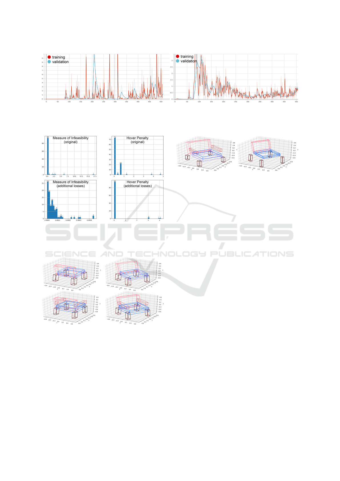
Figure 8: Loss development of the Measure of Infeasibility (left) and the Hover Penalty (right). The total loss is denoted on
the y-axis while the x-axis denotes training steps, with 500 steps corresponding to roughly 35 epochs. The range of each axis
spans to the maximum value found. Mild smoothing has been applied to the graphs, with the original data being hinted at in
the background.
Figure 9: Histograms comparing the Measure of Infeasibil-
ity and Hover Penalty of 100 samples taken before and after
applying the additional losses. The absolute Measure of In-
feasibility or Hover Penalty is shown on the x-axis and the
number of affected samples is shown on the y-axis.
Figure 10: Comparison of two cases of a high Measure of
Infeasibility. The sample in the top row is a result of the
original, unaltered implementation of StructureNet and re-
ceives a Measure of Infeasibility of 17.21. The sample in
the bottom row is a result of the implementation of Struc-
tureNet that includes the new losses and receives a Measure
of Infeasibility of 4.45 · 10
−4
. Both samples were taken af-
ter 35 epochs of training.
primary necessity. An ablation study could also help
to clarify the effects of the individual losses.
Training Duration: Due to additional overhead
caused by the new losses, the training duration
Figure 11: Comparison of two cases of a high Hover
Penalty. The left case is a result of the original, unal-
tered implementation of StructureNet and receives a Hover
Penalty of 4.79. The right case is a result of including the
new losses and receives a Hover Penalty of 3.03. Both
samples were taken after 35 epochs of training. Note that
what can be considered a high Hover Penalty depends on
the overall scale of the shape.
increased significantly. Reducing the performance
impact of the changes is a crucial venue for future
work. This includes more sophisticated initial guess
and faster minimization routines. An improved
interface calculation routine could also help.
Interface Computation: Further necessary
improvements to the interface calculation routine are
related to interface quality. The interfaces resulting
from the current algorithm are arbitrary due to the
random selection of which part to cut into. An
example of three possible outcomes resulting from
the same intersecting geometry is given in Figure 12.
This can have a drastic impact on the Measure of
Infeasibility. An improved solution should provide
deterministic, consistent results and better reflect
human intent. Additionally, it should also try to
minimize the number of triangles used to represent
the interfaces to reduce the optimization time.
Point Clouds: The current handling of point
clouds causes a loss of geometric detail. By separat-
ing the implementation into a bounding box version
and a point cloud version, the geometric data could
be exploited more efficiently.
Materials: We do not support parts of varying
materials. Respecting material properties when
Extending StructureNet to Generate Physically Feasible 3D Shapes
227

Figure 12: Three possible sets of interfaces resulting from
the same geometry. The result depends on which part the
intersection volume is cut out of. Since this is a random
decision, the results are arbitrary. Note that the Measure of
Infeasibility of the leftmost case is lower than the rest due
to neither of the top parts resting on the bottom part.
calculating part weights and friction properties
would yield more realistic results. This includes the
assumption that materials have a uniform density,
which is not always the case in the real world. Our
implementation also ignores deformable parts.
Support Structures: The current solution does
not account for parts being held together by support
structures like screws or bolts, which are common
in the real world. Optimally, a certain amount of
tension forces that could be provided this way should
be granted without reducing the physical feasibility.
Data Sets: Lastly, our extended approach has
only been tested on the PartNet chair data. Further
testing on different data sets is necessary to assess the
general applicability of the method.
8 CONCLUSIONS
In this paper, we have shown an initial step towards
including physical feasibility in the generation of 3D
shapes using StructureNet. While the demonstrated
effects of the Measure of Infeasibility are small, likely
due to the limited training time, significant improve-
ments due to the Hover Penalty are already notice-
able. Further work needs to focus on additional train-
ing, reducing training duration and making the Mea-
sure of Infeasibility more predictable.
REFERENCES
Barequet, G. and Har-peled, S. (2001). Efficiently approxi-
mating the minimum-volume bounding box of a point
set in three dimensions. In In Proc. 10th ACM-SIAM
Sympos. Discrete Algorithms, pages 38–91.
Conn, A. R., Gould, N. I. M., and Toint, P. L. (2000). Trust
Region Methods. Society for Industrial and Applied
Mathematics.
Goodfellow, I., Bengio, Y., and Courville, A. (2016). Deep
Learning. MIT Press.
Kalogerakis, E., Chaudhuri, S., Koller, D., and Koltun, V.
(2012). A Probabilistic Model of Component-Based
Shape Synthesis. ACM Transactions on Graphics,
31(4).
Kingma, D. P. and Welling, M. (2013). Auto-Encoding
Variational Bayes.
Laidlaw, D. H., Trumbore, W. B., and Hughes, J. F. (1986).
Constructive Solid Geometry for Polyhedral Objects.
In Computer Graphics (Proceedings of SIGGRAPH
’86), volume 20, pages 161–170.
Ma, C., Huang, H., Sheffer, A., Kalogerakis, E., and Wang,
R. (2014). Analogy-Driven 3D Style Transfer. In Eu-
rographics 2014, pages 175–184.
Mo, K., Guerrero, P., Yi, L., Su, H., Wonka, P., Mi-
tra, N., and Guibas, L. (2019a). Structurenet: Hi-
erarchical graph networks for 3d shape generation.
ACM Transactions on Graphics (TOG), Siggraph Asia
2019, 38(6):Article 242.
Mo, K., Zhu, S., Chang, A. X., Yi, L., Tripathi, S., Guibas,
L. J., and Su, H. (2019b). PartNet: A large-scale
benchmark for fine-grained and hierarchical part-level
3D object understanding. In The IEEE Conference on
Computer Vision and Pattern Recognition (CVPR).
Pr
´
evost, R., Whiting, E., Lefebvre, S., and Sorkine-
Hornung, O. (2013). Make It Stand: Balancing Shapes
for 3D Fabrication. ACM Trans. Graph., 32(4).
Stava, O., Vanek, J., Benes, B., Carr, N., and M
ˇ
ech, R.
(2012). Stress Relief: Improving Structural Strength
of 3D Printable Objects. ACM Trans. Graph., 31(4).
Whiting, E., Ochsendorf, J., and Durand, F. (2009). Proce-
dural Modeling of Structurally-Sound Masonry Build-
ings. ACM Trans. Graph., 28(5).
Wu, J., Zhang, C., Xue, T., Freeman, W. T., and Tenenbaum,
J. B. (2016). Learning a Probabilistic Latent Space of
Object Shapes via 3D Generative-Adversarial Model-
ing. In Advances in Neural Information Processing
Systems, pages 82–90.
APPENDIX
The source code is available on GitHub: https://
github.com/Novare/structurenet physf.
GRAPP 2021 - 16th International Conference on Computer Graphics Theory and Applications
228
