
Explainable Reinforcement Learning for Longitudinal Control
Roman Liessner
1
, Jan Dohmen
1
and Marco Wiering
2
1
Dresden Institute of Automobile Engineering, TU Dresden, George-B
¨
ahr-Straße 1, Dresden, Germany
2
Bernoulli Institute for Mathematics, Computer Science and Artificial Intelligence,
University of Groningen, 9747 AG Groningen, The Netherlands
Keywords:
Reinforcement Learning, Explainable AI, Longitudinal Control, SHAP.
Abstract:
Deep Reinforcement Learning (DRL) has the potential to surpass the existing state of the art in various prac-
tical applications. However, as long as learned strategies and performed decisions are difficult to interpret,
DRL will not find its way into safety-relevant fields of application. SHAP values are an approach to overcome
this problem. It is expected that the addition of these values to DRL provides an improved understanding of
the learned action-selection policy. In this paper, the application of a SHAP method for DRL is demonstrated
by means of the OpenAI Gym LongiControl Environment. In this problem, the agent drives an autonomous
vehicle under consideration of speed limits in a single lane route. The controls learned with a DDPG algorithm
are interpreted by a novel approach combining learned actions and SHAP values. The proposed RL-SHAP
representation makes it possible to observe in every time step which features have a positive or negative ef-
fect on the selected action and which influences are negligible. The results show that RL-SHAP values are a
suitable approach to interpret the decisions of the agent.
1 INTRODUCTION
The developments in the field of Deep Reinforcement
Learning (DRL) are impressive. After proving in re-
cent years to be able to learn to play challenging video
games (Mnih et al., 2013) on a partly superhuman
level, DRL has recently been used for engineering and
physical tasks. Examples are the cooling of data cen-
ters (Li et al., 2020), robotics (Gu et al., 2016), the en-
ergy management of hybrid vehicles (Liessner et al.,
2018) and self-driving vehicles (El Sallab et al., 2017;
Kendall et al., 2018).
A big challenge for many real-world applications
is the black-box behavior. After a learning process, it
may not be clear why the DRL agent chooses certain
decisions, whether these really are ’intelligent’ deci-
sions or whether the learning process was suboptimal
and the decisions are sometimes clearly wrong. As
long as it cannot be understood how the decisions are
made, it is unsuitable for use in safety-relevant fields
of application. For this reason, in practice simpler
approaches are often preferred for real-world applica-
tions. This problem therefore leads to a trade-off be-
tween performance and interpretability (Kindermans
et al., 2017; Montavon et al., 2017).
1.1 Related Work
According to Doshi-Velez et al. (Doshi-Velez and
Kim, 2017), Lipton (Lipton, 2016) and Montavon et
al. (Montavon et al., 2017), the main reasons for inter-
pretability are: creating trust for the model; checking
whether a model works as expected; improving the
model by comparing it with domain-specific knowl-
edge; and deriving findings from the model.
At the moment most attempts towards inter-
pretable Reinforcement Learning (RL) require a non-
neural network representation of the policy such as a
tree-based policy (Brown and Petrik, 2018), the use
of Genetic Programming for Reinforcement Learning
(Hein et al., 2018), or Programmatically Interpretable
Reinforcement Learning (Verma et al., 2018). These
approaches can therefore not take advantage of the
great progress made in combining RL and neural net-
works. Our goal is to justify the agent’s behavior
while not having to do without established and com-
mon DRL methods such as Deep Deterministic Policy
Gradient (DDPG) (Lillicrap et al., 2015).
In the field of supervised learning, promising ap-
proaches such as SHAP (Lundberg et al., 2017) have
become widespread for improving the interpretability
of learned models. Rizzo et al. show in (Rizzo et al.,
874
Liessner, R., Dohmen, J. and Wiering, M.
Explainable Reinforcement Learning for Longitudinal Control.
DOI: 10.5220/0010256208740881
In Proceedings of the 13th International Conference on Agents and Artificial Intelligence (ICAART 2021) - Volume 2, pages 874-881
ISBN: 978-989-758-484-8
Copyright
c
2021 by SCITEPRESS – Science and Technology Publications, Lda. All r ights reserved

2019) the use of SHAP for an RL traffic signal control
problem with discrete actions. SHAP made it possible
to gain insight into the learned policy for this prob-
lem, although overfitting and unintuitive explanations
were mentioned as remaining issues.
1.2 Contributions of This Paper
In this paper, first the necessity of interpretability for
solving particular RL problems is explained. Then
a particular approach for this challenge is developed
and demonstrated with an example. For this purpose
a suitable method for increasing the intelligibility of
machine learning models is selected. We will demon-
strate how policies learned using actor-critic algo-
rithms can be analyzed with the SHAP method origi-
nating from supervised learning. As an experiment to
illustrate the approach, a DDPG RL algorithm is used
to train an agent for the OpenAI Gym LongiControl
environment. The subsequent analysis of the agent
provides information on how the individual features
of an environmental state contribute to the choice of a
particular action. Finally, a new RL-SHAP represen-
tation method is introduced that helps to increase the
interpretability, and its effectiveness is demonstrated
using the LongiControl example.
1.3 Structure of This Paper
In the following section, the essential basics of DRL
are clarified. With regard to the creation of inter-
pretability, the use of SHAP values will be discussed.
Section 3 introduces a concrete application case for
DRL by means of a vehicle longitudinal control prob-
lem. This includes the definition of the agent, the
environment and the realization of interpretability.
In Section 4 the procedure of interpretable RL is
schematically presented. In Section 5 the results are
shown and analyzed. This is followed by the conclu-
sions in Section 6.
2 BACKGROUND
The proposed methodology applies a method from In-
terpretable Machine Learning, which is used in Su-
pervised Learning, to Reinforcement Learning. Since
this is the most important novelty value, Reinforce-
ment Learning will first be explained and then the
SHAP method that will be used to make the action-
selection policy intelligible will be described.
2.1 Reinforcement Learning
Reinforcement Learning is a direct approach to learn
from interactions with an environment in order to
achieve a defined goal. In this context, the learner and
decision maker is referred to as the agent, whereas the
part it is interacting with is called the environment.
The interaction is taking place in a continuous man-
ner so that the agent selects an action A
t
at each time
step t, and the environment presents the new situation
to the agent in the form of a state S
t+1
. Responding
to the agent’s action, the environment also returns re-
wards R
t+1
in the form of a numerical scalar value.
The agent seeks to maximize the obtained rewards
over time (Sutton and Barto, 2018).
2.1.1 Policy
The policy is what characterizes the agent’s be-
haviour. More formally the policy is a probabilistic
(or deterministic) mapping from states to actions:
π(a|s) = P(A
t
= a|S
t
= s) (1)
2.1.2 Goals and Rewards
In Reinforcement Learning, the agent’s goal is for-
malized in the form of a special signal called a reward,
which is transferred from the environment to the agent
at each time step using a reward function. Basically,
the target of the agent is to maximize the expected to-
tal amount of scalar rewards g
t
= E(
∑
∞
k=0
γ
k
R
t+1+k
|S
t
)
it receives when it is in state S
t
. This quantity, g
t
is
known as the gain or return, and the discount factor
γ ∈ [0, 1] is used to give more importance to earlier
obtained rewards. This results in maximizing not the
immediate reward, but the cumulative reward.
2.1.3 Value Functions
The reward R
t+1
is obtained after performing action
A
t
in the current time step. In RL, the goal is to find a
strategy that maximizes the expected long-term value.
To learn this expected value, Value Functions Q(s, a)
are used and updated. These contain the expected re-
turn E[·] starting in state S
t
, performing action A
t
and
then following policy π. For a Markov Decision Pro-
cess (MDP) we can define:
Q(s, a) = E
"
∞
∑
k=0
γ
k
R
t+k+1
S
t
= s; A
t
= a
#
(2)
2.1.4 Q-Learning
Many popular Reinforcement Learning algorithms
are based on the direct learning of Q-values. One of
Explainable Reinforcement Learning for Longitudinal Control
875
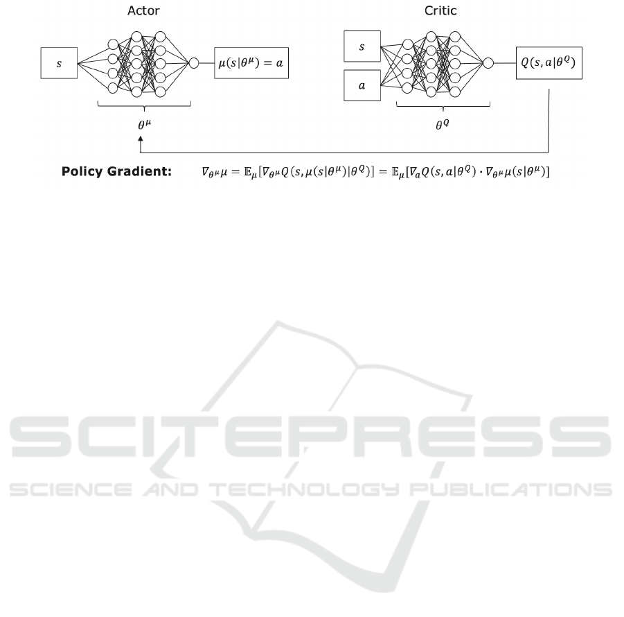
Figure 1: Actor-critic network.
the simplest is Q-Learning (Watkins, 1989). The up-
date rule after an experience tuple (S
t
, A
t
, R
t+1
, S
t+1
)
is as follows:
Q(S
t
, A
t
) ←(1 − α)Q(S
t
, A
t
)
+ α(R
t+1
+ γmax
a
0
Q(S
t+1
, a
0
)) (3)
The update of the Q-function is controlled by the
learning rate α. A greedy deterministic policy can at
all times be derived from the Q-function:
π(S
t
) = argmax
a
Q(S
t
, a) (4)
2.2 Deep Deterministic Policy Gradient
(DDPG)
Finding the optimal action requires an efficient eval-
uation of the Q-function. While this is simple for
discrete and small action spaces (all action values
are calculated and the one with the highest value is
selected), the problem becomes complex if the ac-
tion space is continuous. In many applications such
as robotics and energy management, discretization of
the action space is not desirable, as this can have a
negative impact on the quality of the solution and
at the same time requires large amounts of memory
and computing power in the case of a fine discretiza-
tion. Lillicrap et al. (Lillicrap et al., 2015) presented
an algorithm called DDPG, which is able to solve
continuous-action problems by combining RL with
neural networks. In contrast to Q-Learning, an actor-
critic architecture is used in which the actor is a neural
network that maps from the state to the (continuous)
action. The critic network approximates the Q-value
using the state and action as inputs. The two networks
are illustrated in Figure 1.
The critic continuously updates the Q-Function,
which is called Q
φ
in this context. Additionally a sec-
ond network is used for the actor: π
θ
. The adaptable
parameters φ and θ are updated using experiences by
minimizing a cost function. The cost function for the
Critic given an experience is:
L
critic
= (R
t+1
+ γQ
φ
(S
t+1
, π
θ
(S
t+1
)) − Q
φ
(S
t
, A
t
))
2
(5)
DDPG uses an explicit policy defined by the actor
network π
θ
. Since Q
φ
is a differentiable network, π
θ
can be trained in such a way that it maximizes Q
φ
by
minimizing L
actor
:
L
actor
= −Q
φ
(S
t
, π
θ
(S
t
)) (6)
This has the goal to change the action of the pol-
icy for a state so that the Q-value would increase (Lil-
licrap et al., 2015).
2.3 Interpretability
As discussed in (Lipton, 2016), approaches to cre-
ating interpretability can be divided into two main
groups: Model transparency and post-hoc inter-
pretability. While the former tries to explain the
model structure, the post-hoc interpretability is used
to understand why the model works. Although the
multitude of calculation steps can be understood
within deep learning, no gain in knowledge for the
model can be expected from this. Post-hoc inter-
pretability is therefore of greater interest.
2.3.1 Shapley Values
Utilizing Shapley values is a solution concept of co-
operative game theory. Cooperative game theory in-
vestigates how participants in a game can maximize
their own value by forming coalitions. The goal is to
find a coalition and a distribution of the profits of this
coalition where it is not worthwhile for any player to
form another coalition. Shapley values provide a so-
lution for this. It depends on the contributions of a
player to all possible coalitions. By considering the
marginal contribution in each possible subset of the
coalition, the Shapley values decompose the totals in
each player’s payoff and represent the only solution
that meets the properties of efficiency, linearity, and
symmetry (Shapley, 1953).
ICAART 2021 - 13th International Conference on Agents and Artificial Intelligence
876
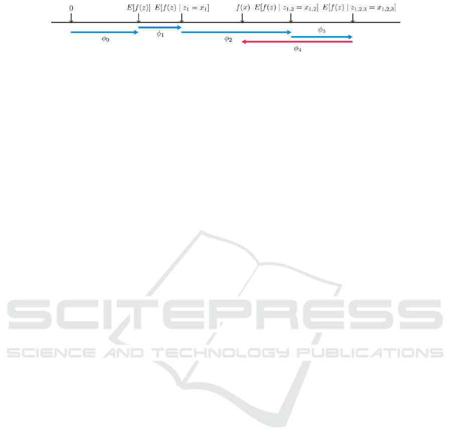
Figure 2: SHAP (SHapley Additive exPlanation) values assign to each attribute the difference in the expected model predic-
tion. These values explain the transition from the base value E[f(z)], which would be predicted if no features were known, to
the actual output f(x) (Lundberg et al., 2017).
2.3.2 SHAP
SHAP (SHapley Additive exPlanations) (Lundberg
et al., 2017) provides a game-theoretical approach to
explain machine learning model outputs. It is an addi-
tive feature attribution method to explain the output of
any machine learning model. SHAP assigns each fea-
ture an importance value for a particular prediction. It
combines optimal credit allocation and local explana-
tions utilizing classical Shapley values. The additive
in the name emphasizes an important property. The
sum of the SHAP values results in the prediction of
the model. The additivity is shown in Figure 2 and
can be described as follows.
f (x) ≈ g(x
0
) = φ
0
+
M
∑
i=1
φ
i
x
0
i
(7)
Where f (x) is the original model, g(x) a simplified
explanation model, x
0
i
the simplified input, such that
x = h
x
(x
0
). The base rate φ
0
= f (h
x
(0)) represents the
model output when all simplified inputs are missing.
3 EXPERIMENTAL SETUP
Since the new method is best explained using an ex-
ample, the experimental setup is presented next. Au-
tonomous vehicles offer the potential to increase road
safety, consume less energy for mobility and make
traffic more efficient (Gr
¨
undl, 2005; Radke, 2013).
In the following, the longitudinal vehicle control
problem will be examined in more detail and opti-
mized for energy efficiency using a DRL algorithm.
On the basis of this relevant practical example, the
advantages of an interpretable model are described.
3.1 Longitudinal Control
It is the aim that a vehicle completes a single-lane
route in a given time as energy-efficient as possible.
In summary, this corresponds to the minimization of
the total energy E used in the interval t
0
≤ t ≤ T as a
function of acceleration a and power P:
minimize
a
E =
Z
T
t
0
P(t, a(t))dt . (8)
In addition, the aim is to maintain speed and ac-
celeration limits and to ensure comfortable driving.
3.2 RL Environment
The LongiControl Environment has been used for an
experimental investigation (Dohmen et al., 2020). In
this example, the vehicle control is represented by the
agent and the route is represented by the environment.
The latter must reflect external influences and pro-
vides feedback for the agent’s actions.
The driving environment is modelled in such a
way that the total distance is arbitrarily long and ran-
domly positioned speed limits specify an arbitrary
permissible velocity. This can be considered equiva-
lent to stochastically modelled traffic. Up to 150 m in
advance, the vehicle driver receives information about
up to two upcoming speed limits and their distance to
the current position, so that a forward-looking driving
strategy is possible. The result is a continuous control
problem, with actions A ∈ R and states S ∈ R
7
.
3.2.1 Action
The agent selects a normalized action in the value
range [-1,1]. The agent can thus choose between
a condition-dependent maximum deceleration and a
maximum acceleration of the vehicle.
3.2.2 State Representation
The features of the state must provide the agent with
all the necessary information to enable a goal-oriented
learning process. The 7 individual features and their
meaning are listed in Table 1.
3.2.3 Reward Function
In the following, the reward function that combines
several objectives is presented. The combined reward
Explainable Reinforcement Learning for Longitudinal Control
877

Table 1: Meaning of the state features.
Feature Meaning
v(t) Vehicles’ current velocity
a
prev
(t) Vehicle acceleration of last time step
v
lim
(t) Current speed limit
v
lim, f ut
(t) The next two speed limits
d
v
lim, f ut
(t) Distances to next 2 speed limits
function consists of four elements with:
r
f orward
(t) = ξ
f orward
×
|v(t) − v
lim
(t)|
v
lim
(t)
r
energy
(t) = ξ
energy
×
ˆ
E
r
jerk
(t) = ξ
jerk
×
|a(t) − a
prev
(t)|
∆t
r
sa f e
(t) = ξ
sa f e
×
(
0 v(t) ≤ v
lim
(t)
1 v(t) > v
lim
(t)
.
Where r
f orward
(t) is the penalty for slow driving,
r
energy
(t) the penalty for energy consumption, r
jerk
(t)
the penalty for jerk and r
sa f e
(t) the penalty for speed-
ing. ξ
∗
are the weighting parameters for the reward
shares. Note that the terms are used as penalties, so
that the learning algorithm minimizes their amount.
The selected weights are all set to 1.0 except for
ξ
energy
(t) which is set to 0.5.
3.3 RL Agent
DDPG (Lillicrap et al., 2015) was chosen as the deep
RL algorithm. The actor-critic implementation is es-
pecially oriented to the version of (Lillicrap et al.,
2015). The DDPG hyperparameters were optimized
using some preliminary experiments and are as fol-
lows: Batch Size = 64. Replay Buffer Size = 10
6
.
Optimizer = Adam Actor Learning Rate = 1 × 10
−5
.
Critic Learning Rate = 1 × 10
−3
. Soft Replacement =
0.001. Discount Factor γ = 0.995. Actor Architecture
= 2 ReLU layers
`
a 256 neurons. Critic Architecture =
2 ReLU layers
`
a 256 neurons.
4 METHOD
The newly presented method consists of four steps. In
the first step the training of an RL agent is required.
The trained agent can then be tested on a trajectory
and the resulting state features and actions will be an-
alyzed by showing diagrams that offer a clear visu-
alization of the reason for selecting an action. These
steps will be explained in more detail in the following
subsections.
4.1 DRL Agent: Training
The training of the DRL agent can be done in the
usual way. There are no explicit training requirements
for the application of the interpretation methodology
presented here, although we focus on actor-critic RL
algorithms. As soon as the agent reaches a particular
performance, the next processing step is performed.
4.2 DRL Agent: Testing
After the training process is stopped, the second step
follows, the testing of the agent. From this point on
only the actor network of the DRL agent is of interest,
which maps the state features to an action.
After the neural network of interest has been de-
termined, For analysing the actor, the question arises
which input values should be used for the test. The-
oretically, random input values would be possible.
However, these would possibly show combinations
for which the DRL agent was not trained and thus vi-
olate the model validity of the actor. In the procedure
presented here, the agent is confronted with new sce-
narios in the LongiControl environment. Since the
agent was trained on stochastically generated tracks
of this environment, this is highly suitable for the test-
ing phase. The resulting state and action sequences
are stored and used for the following evaluation.
4.3 SHAP Values
After the test run the next step is to calculate the
SHAP values. For this purpose an explainer is ap-
proximated from the tensorflow actor network and the
state sequence of the test run (Shrikumar et al., 2017).
The explainer is used to calculate the SHAP val-
ues and the base rate from the state sequence. The
base rate is the model output which is calculated if
the input variables of the neural network are unknown
(not used). The sum of the individual SHAP values
per state and the base rate approximates the action of
the actor (model output).
4.4 RL-SHAP Diagram
The individual examination of some time steps can
provide initial feedback. The user can compare these
results with his/her expectations previously derived
from expert knowledge. However, since it is difficult
to look at the individual examples and to recognize
the long-term effects of the state-action combination,
the entire course of the state variables can be plotted.
For this purpose the actions and state features during
the test process are shown in Figure 3.
ICAART 2021 - 13th International Conference on Agents and Artificial Intelligence
878
In order to improve the intelligibility of such fig-
ures, additional information for the SHAP values will
be shown using colors at the appropriate position. In
this paper a color scale from blue to gray to red is cho-
sen for this purpose. The color scale is normalized to
the action range of the agent (here [-1, 1]) and colors
are used to show the impact of a specific feature on
the selected action. The workings of our approach,
called RL-SHAP diagrams, will be further explained
in the following section.
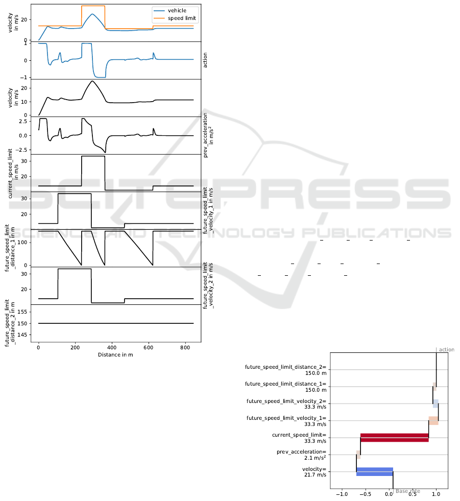
Figure 3: Action and input features over a test route.
5 RESULT
After the description of the agent, the environment
and the interpretation method, the behavior learned
by the agent is interpreted in the following using the
LongiControl Environment as an example.
5.1 Resulting Course
In the first part of the result analysis, the various dia-
grams of Figure 3 will be explained. Figure 3 shows
9 signal courses over the route. The first one shows
the speed of the vehicle in blue and the speed limit
in orange. This representation would not have been
mandatory, since these two pieces of information are
shown in the following diagrams. Nevertheless, the
representation facilitates the understanding. In the
second diagram the course of the agent’s action fol-
lows. This is limited to the range between -1 and
1. Here +1 stands for a maximum positive and -1
for a maximum negative acceleration (deceleration).
The following diagrams show the 7 feature courses
that are included in the state representation. Based on
these, the actor network determines the action.
The third diagram shows the velocity of the vehi-
cle. The fourth diagram shows the acceleration of the
vehicle in the previous step. This value is necessary
to calculate the vehicle’s jerk. In the fifth diagram the
course of the current speed limit is illustrated. The 6th
and 7th diagrams contain information about the next
speed limit. The 6th diagram shows the speed of the
next speed limit and the 7th the distance to the next
speed limit. In the 8th and 9th diagrams the informa-
tion about the next but one speed limit is shown.
The two values for the next but one speed limit
only take effect if there are two speed changes within
the next 150 m. Since this is not the case in
the example, future speed limit distance 2 always re-
mains at the maximum sensor range of 150 m. The
value future speed limit velocity 2 is set equal to fu-
ture speed limit velocity 1 in this case.
The diagram is informative as it shows the input
variables and output variables of the agent. However,
it is not clear how the individual features affect the
result. Therefore, the next step is to show our new
representation of the RL-SHAP values.
Figure 4: SHAP values at 270 m of the test track.
Explainable Reinforcement Learning for Longitudinal Control
879
5.2 RL-SHAP Diagram
Figure 4 shows the SHAP values and the action of the
agent for a single state. In this example the base rate
has a value of 0.08. The SHAP value for the feature
velocity, −0.78, is added to this value. This is fol-
lowed by the SHAP value for the previous accelera-
tion, 0.09. The SHAP value for the current speed limit
adds 1.45 to the summed value and so on. The sum of
the base rate and the seven SHAP values equals 1.0
and corresponds approximately to the action of the
agent (note that a simpler explanation model is used
to compute the SHAP values).
From this example it can be derived that the fea-
ture current speed limit has the largest impact and the
feature future speed limit distance 2 has the least im-
pact on the resulting action for the given state. From
this, we can simply deduce that the agent is fully ac-
celerating mainly because of the high speed limit.
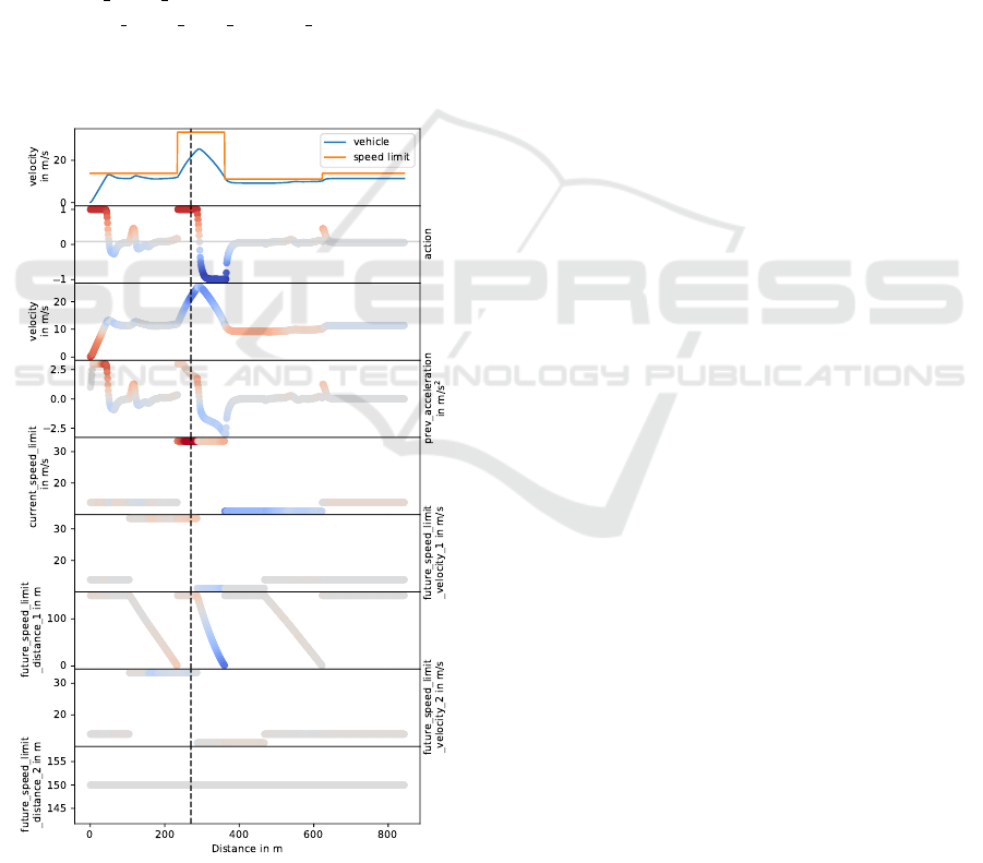
Figure 5: RL-SHAP Diagram of Figure 3. The vertical
dashed line highlights the state analyzed in Figure 4.
After having analyzed the action-selection process
for a single state, we will now examine a longer trajec-
tory. Figure 5 shows the newly introduced RL-SHAP
diagram to get an even more comprehensive insight
into the decision-making process. Compared to the
diagram in Figure 3, further information is shown by
the use of colors. In diagrams 3 - 9 the information
of the state is shown as before. As additional infor-
mation the influence of this feature (SHAP value) on
the selected action is highlighted with the used col-
ors. In the second diagram the action of the agent is
also highlighted in color. The grey horizontal line in-
dicates the base rate. As explained before, this is the
action that is selected when the state is unknown.
As mentioned before, a red coloring of a feature
means that this feature increases the value for the ac-
tion. This is clearly shown by the velocity in the 3rd
diagram within the first 70 m. The agent accelerates
strongly to reach a speed close to the speed limit. Af-
ter that the SHAP value decreases and thus the effect
of this feature on the action, which can be seen by the
change of the color from red to grey. In general blue
values are shown for high velocities and red values
are shown for low velocities. This means the agent
tries to keep a particular average speed.
In comparison, diagrams 8 and 9 of Figure 5 are
mostly grey. This means that the information regard-
ing the next but one speed limit is only slightly in-
cluded in the agent’s decision. Therefore, this feature
seems less important for the agent.
A mix of grey, blue and slightly red influences
can be seen in the 7th diagram. In this diagram the
distance to the next speed limit is shown. If a new
speed limit which is lower than the current one fol-
lows shortly, this feature has a decelerating effect on
the vehicle. This can be seen in the range of blue
values around 300 m distance. The reduction of the
action is largely due to this feature.
Another mix of red and blue influences (positive
and negative SHAP values) can be seen at the current
speed limit. The sometimes strong emphasis of the
blue and red color implies that this feature informa-
tion has a great impact on the action. As soon as the
speed limit jumps to 33.3 m/s at about 250 m, the in-
fluence of this feature increases the action.
Finally, the 4th diagram shows that the previous
acceleration causes some kind of inertia. When the
vehicle was accelerating, this feature also increases
the current acceleration. This can be explained by ex-
amining the penalty for the jerk, in which large devi-
ations in acceleration are punished.
The previous analysis shows that this type of dis-
play makes it possible to clearly see in every time step
which features have a positive or negative effect on
the action and which influences are negligible. On the
basis of these findings, contradictions can be identi-
ICAART 2021 - 13th International Conference on Agents and Artificial Intelligence
880

fied in comparison to expert knowledge. If, for exam-
ple, the agent would increase the action (acceleration)
when the velocity is very large, this would be a strong
indicator of misbehavior.
6 CONCLUSION
The goal of this work was to develop a methodol-
ogy to explain how a trained Reinforcement Learning
agent selects its action in a particular situation. For
this purpose, SHAP values were calculated for the dif-
ferent input features and the effect of each feature on
the selected action was shown in a novel RL-SHAP
diagram representation. The proposed method for ex-
plainable RL was tested using the LongiControl envi-
ronment solved using the DDPG DRL algorithm.
The results show that the RL-SHAP representa-
tion clarifies which state features have a positive, neg-
ative or negligible influence on the action. Our anal-
ysis of the behavior of the agent on a test trajectory
showed that the contributions of the different state
features can be logically explained given some do-
main knowledge. We can therefore conclude that the
use of SHAP and its integration within RL is helpful
to explain the decision-making process of the agent.
As future work, it would be interesting to study
if prior human expert knowledge can be inserted in
the agent using the same RL-SHAP representation.
Finally, we want to study methods that can explain
the decision-making process of DRL agents in high-
dimensional input spaces.
REFERENCES
Brown, A. and Petrik, M. (2018). Interpretable rein-
forcement learning with ensemble methods. CoRR,
abs/1809.06995.
Dohmen, J. et al. (2020). Longicontrol: A reinforcement
learning environment for longitudinal vehicle control.
Researchgate.
Doshi-Velez, F. and Kim, B. (2017). Towards a rigor-
ous science of interpretable machine learning. CoRR.
https://arxiv.org/abs/1702.08608.
El Sallab, A. et al. (2017). Deep reinforcement learning
framework for autonomous driving. CoRR. http:
//arxiv.org/abs/1704.02532.
Gr
¨
undl, M. (2005). Fehler und Fehlverhalten als Ur-
sache von Verkehrsunf
¨
allen und Konsequenzen f
¨
ur
das Unfallvermeidungspotenzial und die Gestaltung
von Fahrerassistenzsystemen. PhD thesis, Universit
¨
at
Regensburg.
Gu, S. et al. (2016). Q-prop: Sample-efficient policy gradi-
ent with an off-policy critic. CoRR. http://arxiv.org/
abs/1611.02247.
Hein, D. et al. (2018). Interpretable policies for rein-
forcement learning by genetic programming. CoRR,
abs/1712.04170.
Kendall, A. et al. (2018). Learning to drive in a day. https:
//arxiv.org/abs/1807.00412.
Kindermans, P. et al. (2017). The (un)reliability of saliency
methods. https://arxiv.org/abs/1711.00867.
Li, Y. et al. (2020). Transforming cooling optimization
for green data center via deep reinforcement learning.
IEEE Transactions on Cybernetics, 50(5):2002–2013.
Liessner, R. et al. (2018). Deep reinforcement learning for
advanced energy management of hybrid electric ve-
hicles. 10th International Conference on Agents and
Artificial Intelligence.
Lillicrap, T. et al. (2015). Continuous control with deep
reinforcement learning. CoRR. http://arxiv.org/abs/
1509.02971.
Lipton, Z. C. (2016). The mythos of model interpretability.
CoRR. http://arxiv.org/abs/1606.03490.
Lundberg, S. et al. (2017). A unified approach to inter-
preting model predictions. In Advances in Neural In-
formation Processing Systems 30, pages 4765–4774.
Curran Associates, Inc.
Mnih, V. et al. (2013). Playing atari with deep reinforce-
ment learning. CoRR. http://arxiv.org/abs/1312.5602.
Montavon, G. et al. (2017). Methods for interpreting and
understanding deep neural networks. CoRR. http://
arxiv.org/abs/1706.07979.
Radke, T. (2013). Energieoptimale L
¨
angsf
¨
uhrung von
Kraftfahrzeugen durch Einsatz vorausschauender
Fahrstrategien. PhD thesis, Karlsruhe Institute of
Technology (KIT).
Rizzo, S. et al. (2019). Reinforcement learning with ex-
plainability for traffic signal control. In 2019 IEEE In-
telligent Transportation Systems Conference (ITSC),
pages 3567–3572.
Shapley, L. (1953). A value for n-persons games. Contri-
butions to the Theory of Games 2, 28:307–317.
Shrikumar, A. et al. (2017). Learning important features
through propagating activation differences. CoRR,
abs/1704.02685.
Sutton, R. S. and Barto, A. G. (2018). Reinforcement Learn-
ing: An Introduction. MIT Press, Cambridge, MA,
USA, 2te edition.
Verma, A. et al. (2018). Programmatically interpretable re-
inforcement learning. CoRR, abs/1804.02477.
Watkins, C. J. C. H. (1989). Learning from delayed rewards.
PhD thesis, University of Cambridge.
Explainable Reinforcement Learning for Longitudinal Control
881
