Practical Auto-calibration for Spatial Scene-understanding from
Crowdsourced Dashcamera Videos
Hemang Chawla, Matti Jukola, Shabbir Marzban, Elahe Arani and Bahram Zonooz
Advanced Research Lab, Navinfo Europe, The Netherlands
Keywords:
Vision for Robotics, Crowdsourced Videos, Auto-calibration, Depth Estimation, Ego-motion Estimation.
Abstract:
Spatial scene-understanding, including dense depth and ego-motion estimation, is an important problem in
computer vision for autonomous vehicles and advanced driver assistance systems. Thus, it is beneficial to
design perception modules that can utilize crowdsourced videos collected from arbitrary vehicular onboard or
dashboard cameras. However, the intrinsic parameters corresponding to such cameras are often unknown or
change over time. Typical manual calibration approaches require objects such as a chessboard or additional
scene-specific information. On the other hand, automatic camera calibration does not have such requirements.
Yet, the automatic calibration of dashboard cameras is challenging as forward and planar navigation results
in critical motion sequences with reconstruction ambiguities. Structure reconstruction of complete visual-
sequences that may contain tens of thousands of images is also computationally untenable. Here, we propose
a system for practical monocular onboard camera auto-calibration from crowdsourced videos. We show the
effectiveness of our proposed system on the KITTI raw, Oxford RobotCar, and the crowdsourced D
2
-City
datasets in varying conditions. Finally, we demonstrate its application for accurate monocular dense depth and
ego-motion estimation on uncalibrated videos.
1 INTRODUCTION
Autonomous driving systems have progressed over
the years with advances in visual perception technol-
ogy that enables safer driving. These advances in
computer vision have been possible with the enor-
mous amount of visual data being captured for train-
ing neural networks applied to a variety of scene-
understanding tasks such as dense depth and ego-
motion estimation. Nevertheless, acquiring and an-
notating vehicular onboard sensor data is a costly
process. One of the ways to design generic per-
ception systems for spatial scene-understanding is to
utilize crowdsourced data. Unlike most available
datasets which contain limited hours of visual infor-
mation, exploiting large scale crowdsourced data of-
fers a promising alternative (Dabeer et al., 2017; Gor-
don et al., 2019)
Crowdsourced data is typically collected from
low-cost setups such as monocular dashboard cam-
eras. However, the robustness of modern multi-
view perception systems used in dense depth esti-
mation (Godard et al., 2019), visual odometry (Mur-
Artal et al., 2015), lane detection (Ying and Li, 2016),
object-specific distance estimation (Zhu and Fang,
2019), optical flow computation (Meister et al., 2018),
and so on, depends upon the accuracy of their cam-
era intrinsics. The lack of known camera intrinsics
for crowdsourced data captured from unconstrained
environments prohibits the direct application of exist-
ing approaches. Therefore, it is pertinent to estimate
these parameters, namely focal lengths, optical cen-
ter, and distortion coefficients automatically and ac-
curately. Yet, standard approaches to obtaining these
parameters necessitate the use of calibration equip-
ment such as a chessboard, or are dependent upon the
presence of specific scene geometry such as planes
or lines (Wildenauer and Micusik, 2013). A vari-
ety of approaches to automatically extract the cam-
era intrinsics from a collection of images have also
been proposed. Multi-view geometry based meth-
ods utilize epipolar constraints through feature ex-
traction and matching for auto-calibration (Gherardi
and Fusiello, 2010; Kukelova et al., 2015). How-
ever, for the typical driving scenario with constant
but unknown intrinsics, forward and planar camera
motion results in critical sequences (Steger, 2012;
Wu, 2014). Supervised deep learning methods in-
stead require images with known ground truth (GT)
parameters for training (Lopez et al., 2019; Zhuang
Chawla, H., Jukola, M., Marzban, S., Arani, E. and Zonooz, B.
Practical Auto-calibration for Spatial Scene-understanding from Crowdsourced Dashcamera Videos.
DOI: 10.5220/0010255808690880
In Proceedings of the 16th International Joint Conference on Computer Vision, Imaging and Computer Graphics Theory and Applications (VISIGRAPP 2021) - Volume 5: VISAPP, pages
869-880
ISBN: 978-989-758-488-6
Copyright
c
 2021 by SCITEPRESS – Science and Technology Publications, Lda. All rights reserved
869

et al., 2019). While Structure-from-Motion has also
been used for auto-calibration, its direct application
to long crowdsourced onboard videos is computa-
tionally expensive (Schonberger and Frahm, 2016),
and hence unscalable. This motivates the need for
a practical auto-calibration method for spatial scene-
understanding from unknown dashcameras.
Recently, camera auto-calibration through
Structure-from-Motion (SfM) on sub-sequences
of turns from KITTI raw dataset (Geiger et al.,
2012) was proposed for 3D positioning of traffic
signs (Chawla et al., 2020a). However, the method
was limited by the need for Global Positioning
System (GPS) information corresponding to each
image in the dataset. The GPS information may not
always be available, or may be collected at a different
frequency than the images, and may be noisy. Fur-
thermore, no analysis was performed on the kind of
sub-sequences necessary for successful and accurate
calibration. Typical visibility of ego-vehicle in the
onboard images also poses a problem to the direct
application of SfM. Therefore, scalable accurate
auto-calibration from onboard visual sequences
remains a challenging problem.
In this paper, we present a practical method for
extracting camera parameters including focal lengths,
principal point, and radial distortion (barrel and pin-
cushion) coefficients from a sequence of images col-
lected using only an onboard monocular camera. Our
contributions are as follows:
• We analytically demonstrate that the sub-
sequences of images where the vehicle is turning
provide the relevant structure necessary for a
successful auto-calibration.
• We introduce an approach to automatically deter-
mine these turns using the images from the se-
quence themselves.
• We empirically study the relation of the frames
per second (fps) and number of turns in a video
sequence to the calibration performance, showing
that a total ≈ 30 s of sub-sequences are sufficient
for calibration.
• A semantic segmentation network is additionally
used to deal with the variable shape and amount of
visibility of ego-vehicle in the image sequences,
improving the calibration accuracy.
• We validate our proposed system on the KITTI
raw, the Oxford Robotcar (Maddern et al., 2017),
and the D
2
-City (Che et al., 2019) datasets against
state-of-the-art.
• Finally, we demonstrate its application to
chessboard-free dense depth and ego-motion es-
timation on the uncalibrated KITTI Eigen (Eigen
and Fergus, 2015) and Odometry (Zhou et al.,
2017) splits respectively.
2 RELATED WORK
Over the years, multiple ways have been devised to
estimate camera parameters from a collection of im-
ages for which the camera hardware is either un-
known or inaccessible. Methods using two or more
views of the scene have been proposed to estimate
camera focal lengths (Gherardi and Fusiello, 2010).
The principal point is often fixed at the center of
the image, as its calibration is an ill-posed prob-
lem (de Agapito et al., 1998). To estimate radial
distortion coefficients, two-view epipolar geometry
constraints are often used (Kukelova et al., 2015).
Note that forward camera motion is a degenerate
scenario for distortion estimation due to ambiguity
against scene depth. Similarly, planar camera mo-
tion is also a critical calibration sequence (Wu, 2014).
Nevertheless, typical automotive visual data captured
from dashcameras majorly constitute forward motion
on straight paths and a few turns, within a mostly
planar motion. Supervised learning based meth-
ods for camera auto-calibration have also been intro-
duced (Lopez et al., 2019; Zhuang et al., 2019). How-
ever, their applicability is constrained by the variety
of images with different combinations of ground truth
camera parameters used in training. On the other-
hand self-supervised methods (Gordon et al., 2019)
do not achieve similar performance (Chawla et al.,
2020b). SfM has also been utilized to estimate cam-
era parameters from a crowdsourced collection of im-
ages (Schonberger and Frahm, 2016). However, the
reconstruction of a complete long driving sequence
of tens of thousands of images is computationally ex-
pensive, motivating the utilization of a relevant sub-
set of images (Chawla et al., 2020a). Therefore, this
work proposes a practical system for intrinsics auto-
calibration from onboard visual sequences. Our work
can be integrated with the automatic extrinsic calibra-
tion of (Tummala et al., 2019) for obtaining the com-
plete camera calibration.
3 SYSTEM DESIGN
This section describes the components of the pro-
posed practical system for camera auto-calibration us-
ing a crowdsourced sequence of n images captured
from an onboard monocular camera. We represent the
camera parameters using the pinhole camera model
VISAPP 2021 - 16th International Conference on Computer Vision Theory and Applications
870

Sequence
of
Images
Turns
Found?
Merge
Turns
Success?
Camera
Parameters
Unable
to
Calibrate
Y Y
N N
Reconstruct
Each Turn
Turn
Detection
From Images
Section 3.1
Detect
Potential
Turns
Median
Filtering
Compute
Peaks and
Prominences
For each turn
Generate
Image
Triplets
Feature
Extraction
Matching and
Geometric
Verification
Incremental
Reconstruction
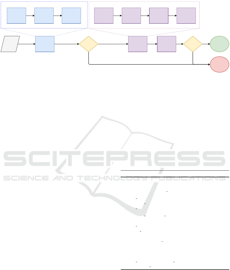
Figure 1: Practical Auto Calibration from on-board visual sequences. The input to the system is represented in gray. The
components of turn detection step (Section 3.1) are shown in blue. The components of the turn reconstruction for parameter
extraction (Section 3.2) are shown in purple.
and a polynomial radial distortion model with two pa-
rameters (Hartley and Zisserman, 2003). The intrinsic
matrix is given by,
K =


f
x
0 c
x
0 f
y
c
y
0 0 1


, (1)
where f
x
and f
y
are the focal lengths, and (c
x
,c
y
) rep-
resents the principal point. The radial distortion is
modeled using a polynomial with two parameters k
1
and k
2
such that,

x
d
y
d

= (1 + k
1
r
2
+ k
2
r
4
)

x
u
y
u

, (2)
where (x
d
,y
d
) and (x
u
,y
u
) represent the distorted and
rectified pixel coordinates respectively, while r is the
distance of the coordinate from the distortion center
(assumed to be the same as the principal point). An
overview of the proposed framework is shown in Fig-
ure 1.
Our system is composed of two broad modules.
The first module is turn detection which outputs a
list of ς sub-sequences corresponding to the turns
in the video. The second module is incremental re-
construction based auto-calibration using these sub-
sequences. This involves building the scene graph
of image pairs with geometrically verified feature
matches. The scene graph is then used to reconstruct
each detected turn within a bundle adjustment frame-
work, followed by a merging of the turns. This allows
to extract the single set of camera parameters from the
captured turn sequences.
Turns are necessary in extracting the camera pa-
rameters for two reasons:
1. As stated earlier, the pure translation and pure for-
ward motion of the camera are degenerate scenar-
ios for auto-calibration of the focal lengths and the
distortion coefficients respectively (Steger, 2012;
Wu, 2014).
2. Moreover, the error in estimating the focal lengths
is bounded by the inverse of the rotation between
the matched frames, as derived in Sec 3.2.
3.1 Turn Detection
Algorithm 1 summarizes the proposed method for
turn detection. This method estimates the respective
median images for the turns present in the full video.
Thereafter for each median image (turn center), k pre-
ceding and succeeding images are collated to form the
turn sub-sequences.
Algorithm 1: Turn Detection.
input : a list of images I
1
...I
n
∈ I
max number of turns ς
output: a list of turn centers
1 turn centers ← []
2 potential tur ns ← []
3 turn magnitudes ← []
4 potential tur ns, turn magnitudes ←
computePotentialTurns(I)
5 turn magnitudes ← medianFilter
(turn magnitudes)
6 peaks, prominences ←
findPeaks(turn magnitudes)
7 peaks.sort(prominences)
8 peaks.reverse()
9 peaks ← peaks [1 : min(ς, len(peaks))]
10 turn centers ← potential turns [peaks ]
11 return tur n centers
To identify potential turns in the complete im-
age sequence, we utilize a heuristic based on
epipoles (Hartley and Zisserman, 2003). The image
sequence is broken into triplets of consecutive im-
ages, and the epipoles are computed for the C
3
2
com-
binations of image pairs. The portions where the ve-
hicle is undergoing pure translation is indicated by
the failure to extract the epipoles. For the remaining
Practical Auto-calibration for Spatial Scene-understanding from Crowdsourced Dashcamera Videos
871

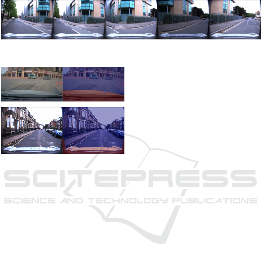
Figure 2: Sample images from a turn detected in the Oxford Robotcar dataset using Algorithm 1. The middle image corre-
sponds to the detected turn median. For visualization, the remaining shown images are selected with a step size of 5 frames
from the sub-sequence.
Figure 3: Masked ego-vehitcle using (Arani et al., 2021).
Left: Input image. Right: Segmented image with masked
ego-vehicle (red) and valid region (blue). Examples from
D
2
-City (top), and Oxford Robotcar (bottom) datasets.
Note the varying shape, angles, and amount of ego-vehicle
visibility. Only the valid region is used during feature ex-
traction and matching for calibration.
portions, the average relative distance of the epipoles
from the image centers is used as an indicator for the
turning magnitude. We filter the estimated potential
turn magnitudes across the sequence for noise, using
a median filter with window size 2 · bk/2c − 1.
Thereafter, we compute the peaks (local maximas)
and the topographic prominences of the potential turn
magnitudes. The prominences, sorted in a descend-
ing order are the proxy for the likelihood of each
peak being a usable turn. Selecting the top ς turns
based on the peak prominences, we construct the sub-
sequences containing 2k + 1 images each. Figure 2
shows a set of sample images from a detected turn in
the Oxford Robotcar dataset.
3.2 Calibration
Given the ς turn sub-sequences, the camera is cali-
brated within a SfM framework. Each turn is incre-
mentally reconstructed, and the models for the turns
are consequently merged to output the final camera
parameters as shown in Figure 1. Utilizing multiple
turns assists in increasing the reliability of the cal-
ibration and accounting for any false positive turn-
detections that may not be successfully reconstructed.
Calibration through SfM involves building a scene
graph for each turn. The images in the turn are the
nodes of this graph, and the validated image pairs with
their inlier feature correspondences are the edges.
This requires extracting features from the images and
matching them across the sequence, followed by a ge-
ometric verification of the matches.
Ego-vehicle Masking. One of the challenges in
crowdsourced dashcamera sequences is the presence
of the ego-vehicle in the images. This impacts the
correspondence search negatively (Schonberger and
Frahm, 2016). Upon sampling several crowdsourced
sequences, we find that they have varying segments
of car dashboard as well as A-pillars visible in the
camera view, making a fixed crop of the images an
infeasible solution. Therefore, we utilize a real-time
semantic segmentation network (Arani et al., 2021)
trained on Mapillary dataset (Neuhold et al., 2017)
for masking out the ego-vehicle (see Figure 3) during
feature extraction.
Reconstruction. After building the scene graph,
we reconstruct each turn within an incremental SfM
framework to output a set of camera poses P ∈ SE(3)
and the scene points X ∈ R
3
(Schonberger and Frahm,
2016).
The Perspective-n-Point (PnP) problem is solved
during turn reconstruction to simultaneously estimate
the camera poses, scene structure, and the camera
parameters, optimized within a bundle adjustment
framework. This uses the correspondences between
the 2D image features and the observed 3D world
points for image registration.
Based on this, we show that the error in estimat-
ing the focal lengths is bounded by the inverse of the
rotation between the matched frames. For simplicity
of derivation, we keep the principal point fixed at the
image center. The camera model maps the observed
world points P
w
to the feature coordinates p
c
of the
rectified image such that,
sp
c
= KR
cw
P
w
+ Kt
cw
, (3)
VISAPP 2021 - 16th International Conference on Computer Vision Theory and Applications
872

where the product of the camera intrinsic matrix K
(Eq. 1) and the rigid camera pose with rotation
R
cw
∈ SO(3) and translation t
cw
∈ R
3
is the projec-
tion matrix, and s denotes scale factor proportional
to the projective depth of the features. The distor-
tion model (Eq. 2) further relates the distorted feature
coordinates with the rectified feature coordinates p
c
.
Accordingly, we can associate the feature matches of
the observed 3D points in any two (i, j) of the m cam-
era views correspondences through
sp
j
= KRK
−1
p
i
+ Kt. (4)
In the scenario of pure translation without any ro-
tation, Eq. 4 reduces to
sp
j
= Kt, (5)
showing that the correspondences cannot be utilized
for calibration. Now consider the scenario where
there is no translation. The feature/pixel shift is then
only determined by the amount of rotation,
p
j
=
KRK
−1
p
i
(KRK
−1
p
i
)
3
, (6)
where the subscript 3 represents the third compo-
nent of the 3 × 1 homogeneous feature coordinates
vector. Having correspondences across overlapping
frames allows for the assumption that relative rotation
is small. Hence, we can write
R = I + r, (7)
where r =


0 r
z
−r
y
−r
z
0 r
x
r
y
−r
x
0


. (8)
To be able to finally derive an analytic expression, we
expand Eq. 6 for r using Taylor series to obtain,
p
j
= p
i
+ (KrK
−1
p
i
) − p
i
(KrK
−1
p
i
)
3
, (9)
where the subscript 3 represents the third component
of the 3 × 1 homogeneous feature coordinates vector.
Since vehicular motion primarily consists of the car
turning about the y axis, we only consider the yaw
r
y
for this derivation. Substituting the camera matrix
from Eq. 1 and the rotation matrix from Eq. 7 in Eq.
9, we obtain
p
j(x)
= − f
x
r
y
− r
y
(p
i(x)
− c
x
)
2
f
x
, (10)
p
j(y)
= −r
y
(p
i(x)
− c
x
)(p
i(y)
− c
y
)
f
x
. (11)
Similar equations can also be written for the estimated
camera parameters and the reprojected feature coordi-
nates. Bundle adjustment minimizes the re-projection
error,
ε =
∑
j
ρ
j



ˆp
j
− p
j


2
2

(12)
=
∑
j
ρ
j

|δp
j(x)
|
2
+ |δp
j(y)
|
2

, (13)
where ρ
j
down-weights the outlier matches, and ˆp
j
=
p
j
+ δp
j
, are the reprojected feature coordinates.
Thus, the parameters to be estimated, focal lengths
ˆ
f
x
,
ˆ
f
y
, camera rotation ˆr
y
, and distortion coefficients
k
1
, k
2
appear implicitly in the error function above.
Since the camera rotation and intrinsics are opti-
mized simultaneously to minimize the re-projection
error, we can assume that the estimated ˆr
y
balances
the estimated camera parameters. For simplicity, we
choose a yaw that at least the features close to the
principal point remain unchanged, where the impact
of distortion is also negligible. Therefore, from Eqs.
10 and 11, we understand
ˆr
y
ˆ
f
x
= r
y
f
x
. (14)
Now we can write the equations for the estimated fea-
ture point coordinates replacing ˆr
y
to obtain,
ˆp
j(x)
= − f
x
r
y
− f
x
r
y
(p
i(x)
− c
x
)
2
ˆ
f
2
x
, (15)
ˆp
j(y)
= − f
x
r
y
(p
i(x)
− c
x
)(p
i(y)
− c
y
)
ˆ
f
2
x
. (16)
Accordingly, by subtracting Eqs. 10 and 11 from Eqs.
15 and 16 respectively, we get the first order approxi-
mation of δp
j
,
δp
j(x)
= 2δ f
x
r
y
(p
i(x)
− c
x
)
2
f
2
x
, (17)
δp
j(y)
= 2δ f
x
r
y
(p
i(x)
− c
x
)(p
i(y)
− c
y
)
f
2
x
. (18)
For the errors |δp
j
(x)|  1 and |δp
j
(y)|  1, we need
to simultaneously satisfy
|δ f
x
| 
f
2
x
2r
y
(p
i(x)
− c
x
)
2
and, (19)
|δ f
x
| 
f
2
x
2r
y
|p
i(x)
− c
x
||p
i(y)
− c
y
|
(20)
with the features closer to the boundary providing the
tightest bound on |δ f
x
|. Since c
x
= w/2 and c
y
= h/2,
we obtain,

δ f
x
δ f
y

|
<
2
max(h,w)

f
2
x
w · r
y
f
2
y
h · r
x

|
. (21)
This result is similar to the Eq. 3 obtained in (Gordon
et al., 2019). Thus the errors in focal lengths f
x
and
Practical Auto-calibration for Spatial Scene-understanding from Crowdsourced Dashcamera Videos
873

f
y
are bounded by the inverse of rotation about the y
and x axes, respectively.
Since the vehicular motion is planar with lim-
ited pitch rotations, we perform the calibration in two
steps:
1. As modern cameras are often equipped with
nearly square pixels, we fix f
x
= f
y
and utilize the
yaw rotations about the y axis to calibrate the fo-
cal lengths. The principal point is also fixed to the
center of the image. This step outputs a common
focal length and the refined distortion coefficients.
2. Thereafter, we relax these assumptions and refine
all the parameters simultaneously within bounds.
This allows to slightly update f
y
and also refine
the principal point to minimize the reprojection
error.
The final output is a set of six parameters namely, fo-
cal lengths f
x
, and f
y
, principal point (c
x
, c
y
), and the
radial distortion coefficients k
1
and k
2
. Thereafter, the
reconstructed models of the turns are merged. Thus,
instead of optimizing the intrinsics as separate param-
eters for each turn, they are estimated as a single set
of constants. In the few scenarios where overlapping
turn sub-sequences may be present, they are also spa-
tially merged and optimized together.
4 EXPERIMENTS
We validate our proposed system for auto-calibration
of onboard cameras on the KITTI raw (Geiger et al.,
2012), the Oxford Robotcar (Maddern et al., 2017),
and the D
2
-city (Che et al., 2019) datasets. Ego-
vehicle is visible in the onboard camera of Oxford
Robotcar and the dashcamera of D
2
-City datasets, re-
spectively. Corresponding GPS information (used in
competing methods) is not availbale for the crowd-
sourced D
2
-City dataset.
We compare our system against (Chawla et al.,
2020a) which uses GPS based turn detection and
SfM for calibration, as well as (Santana-Cedr
´
es et al.,
2017) which relies upon detecting lines, curves and
Hough transform in the scene. We also demonstrate
the necessity of masking the ego-vehicle for accurate
calibration. To further evaluate our proposed system,
we empirically study the impact of the number of
turns used, as well as the frame rate of the videos on
the calibration performance. We show that our sys-
tem is superior to (Santana-Cedr
´
es et al., 2017) as
well as (Chawla et al., 2020a; Chawla et al., 2020b),
which in turn outperforms the self-supervised (Gor-
don et al., 2019). Finally, we demonstrate the ap-
plication of our system for chessboard-free accurate
monocular dense depth and ego-motion estimation on
uncalibrated videos.
4.1 Datasets
KITTI Raw. This dataset contains sequences from
the urban environment in Germany with a right-
hand drive. The images are captured at 10 fps with
the corresponding GPS at 100 Hz. The ground
truth (GT) camera focal lengths, principal point,
and the radial distortion coefficients and model are
available for the different days the data was cap-
tured. The GT camera parameters correspond-
ing to Seq 00 to 02 are { f
x
= 960.115 px, f
y
=
954.891 px,c
x
= 694.792 px,c
y
= 240.355 px,k
1
=
−0.363,k
2
= 0.151}, and for Seq 04 to 10 are { f
x
=
959.198px, f
y
= 952.932 px, c
x
= 694.438 px, c
y
=
241.679 px,k
1
= −0.369, k
2
= 0.158}. Seq 03 is not
present in the raw dataset. Also, the ego-vehicle is not
visible in the captured data.
Oxford Robotcar. This dataset contains sequences
from the urban environment in the United Kingdom
with a left-hand drive. The images are captured at
16 fps, and the GPS at 16 Hz. However, some of
the sequences have poor GPS or even do not have
corresponding GPS available. A single set of GT
camera focal lengths and the principal point is avail-
able for all the recordings, { f
x
= 964.829 px, f
y
=
964.829 px,c
x
= 643.788 px,c
y
= 484.408 px}. In-
stead of the camera distortion model and coefficients,
a look-up table (LUT) is available that contains the
mapping between the rectified and distorted images.
The ego-vehicle is also visible in the captured data.
D
2
-City. This dataset contains crowdsourced se-
quences collected from dashboard cameras onboard
DiDi taxis in China. Therefore, the ego-vehicle is vis-
ible in the captured data. Different sequences have
different amount and shape of this dashboard and A-
pillar visibility. There is no accompanying GPS. The
images are collected at 25 fps across varying road and
traffic conditions. Consequently, no GT camera pa-
rameters are available as well.
4.2 Performance Evaluation
Table 1 summarizes the results of performance eval-
uation of our proposed onboard monocular cam-
era auto-calibration system. We evaluate on ten
KITTI raw sequences 00 to 10 (except sequence
03, which is missing in the dataset), and re-
port the average calibration performance. Further-
more, we evaluate on three sequences from the Ox-
VISAPP 2021 - 16th International Conference on Computer Vision Theory and Applications
874

Table 1: Comparing calibration performance measured through median absolute percentage error and mean SSIM across
datasets. M represents ego-vehicle masking. The best estimates for each parameter on the datasets are highlighted in gray.
Dataset Method ↓ f
x
↓ f
y
↓ c
x
↓ c
y
↓ k
1
↓ k
2
↑ SSIM
µ
KITTI
Raw
(Chawla et al., 2020a) 1.735 0.967 0.884 0.051 11.435 34.488 -
Ours (w/o M) 1.670 0.525 0.717 0.522 11.421 34.034 -
Oxford
(Good GPS)
(Chawla et al., 2020a) 7.065 6.018 0.715 0.151 - - 0.889
Ours (w/o M) 8.068 6.394 1.152 0.433 - - 0.890
Ours (with M) 7.598 6.286 0.587 0.426 - - 0.893
Oxford
(Poor GPS)
(Chawla et al., 2020a) 6.763 6.156 0.418 0.017 - - 0.908
Ours (w/o M) 1.975 0.703 0.513 3.010 - - 0.906
Ours (with M) 1.892 0.361 0.386 2.516 - - 0.909
Oxford
(No GPS)
Ours (w/o M) 13.937 18.956 0.857 1.639 - - 0.897
Ours (with M) 6.610 6.408 1.207 0.549 - - 0.899
ford Robotcar dataset with different GPS qualities,
2014-11-28-12-07-13 with good GPS measure-
ments, 2015-03-13-14-17-00 with poor GPS mea-
surements, and 2015-05-08-10-33-09 without any
accompanying GPS measurements. We repeat each
calibration 5 times are report the median absolute per-
centage error for the estimated focal lengths, princi-
pal point, and the distortion coefficients. Since the
GT distortion model and coefficients are not provided
in the Oxford robotcar dataset, we instead measure
the mean structural similarity (Wang et al., 2004) be-
tween the images rectified using the provided Look-
up-table (LUT) and our estimated parameters. Fi-
nally, we calibrate 10 turn-containing sequences of
30 s each, from the D
2
-City dataset.
We successfully calibrate all sequences except for
KITTI 04 which does not contain any turns. Our
method performs better than (Chawla et al., 2020a)
in all the cases except for Oxford (Good GPS). This
case can be attributed to better turn detection with
good GPS quality used by that method, which is often
not available for crowdsourced data. Also, note that
the calibration is better when using the proposed ego-
vehicle masking. This effect is most pronounced for
Oxford (No GPS) where the focal length errors be-
come nearly half when masking out the ego-vehicle.
The calibration without ego-vehicle masking is less
effective with the presence of ego-vehicle in the im-
ages, as it acts as a watermark and negatively impacts
feature matching (Schonberger and Frahm, 2016),
even with the use of RAndom SAmple Consensus
(RANSAC) (Hartley and Zisserman, 2003).
Following the comparison protocol of (Santana-
Cedr
´
es et al., 2017)
1
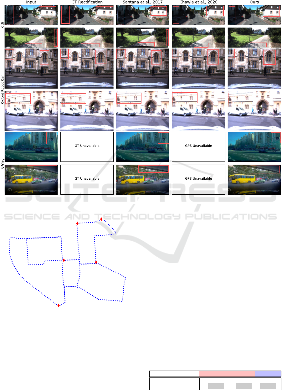
, Figure 4 shows some quali-
tative auto-calibration results comparing our system
against (Chawla et al., 2020a; Santana-Cedr
´
es et al.,
2017). Note that our system performs better, as vis-
ibly demonstrated by the rectified structures. More-
over, our method is applicable even when no GPS
1
http://dev.ipol.im/
∼
asalgado/ipol demo/workshop
perspective/
information is available, as we successfully calibrate
all the selected sequences from D
2
-City. However,
our system relies upon the features in the images and
thus is more suitable for urban driving sequences. Ad-
ditional qualitative results for the dashcamera videos
from D
2
-city can be found in the Appendix.
4.3 Design Evaluation
Here, we further evaluate our proposed system design
for the impact of the number of turns used during cal-
ibration, and the frame rate of the onboard image se-
quence, on the calibration performance. We carry out
these analyses on KITTI sequence 00. For all these
experiments the value of k is set to 30.
For each experiment repeated multiple times, we
report the calibration error metric as the median of
absolute percentage error normalized by the number
of times the calibration was successful. This unitless
metric is used to capture the accuracy as well as the
consistency of the auto-calibration across the afore-
mentioned settings.
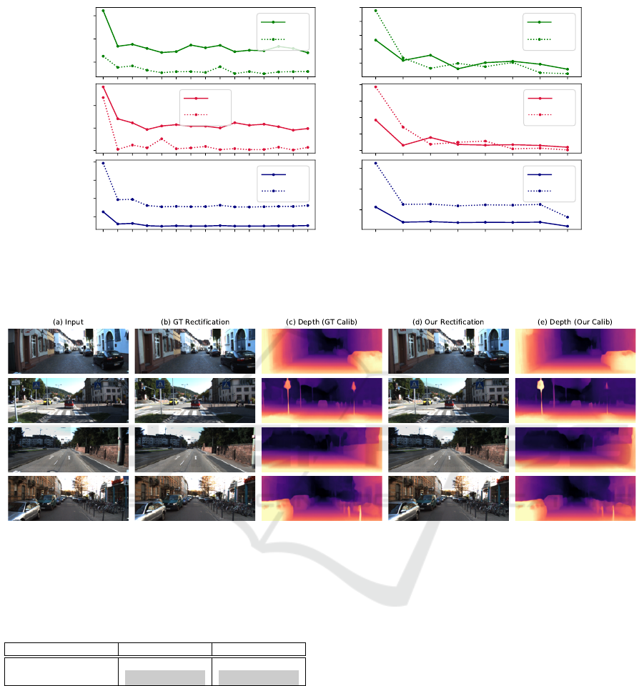
Number of Turns. Here, we study the impact of the
number of turns on the calibration error metric. For
this analysis, we first create a set S
turns
of the top 15
turns (at 10 fps) extracted using Algorithm 1. There-
after, we vary the number of turns j used for cali-
bration by randomly selecting them from S
turns
. We
repeat each experiment 10 times and report the cali-
bration error metric (see Figure 6). Note that the fo-
cal lengths estimation improves up to two turns. The
principal point estimation improves up to four turns.
The distortion coefficients estimation improves up to
five turns. Therefore, successful auto-calibration with
our approach requires a minimum of 5 turns, con-
sisting of only a few hundred (≈300) images. Fig-
ure 5 shows the top 5 of the extracted turns for auto-
calibration of KITTI Sequence 00. This reinforces the
practicality and scalability of our system.
Practical Auto-calibration for Spatial Scene-understanding from Crowdsourced Dashcamera Videos
875

o
:p
so
:p
:O
:
0000000
DO
D
O
O
O
O
O
D
O
O
O
-
o
Figure 4: Qualitative comparison of camera auto-calibration on the KITTI raw (top), the Oxford Robotcar (middle), and the
D
2
-city (bottom) datasets.
Figure 5: Using the top 5 turns for auto-calibration of KITTI
Seq 00. The red diamonds denote the turn centers, and the
dotted blue line is the corresponding GPS trajectory. Note
that our method does not use this GPS trajectory for turn
estimation.
Frame Rate. We study the impact of the frame rate
by sampling the image sequence across a range of
1 fps to 10 fps, and report the calibration metric as
before (see Figure 6). Note that calibration is un-
successful when the frame rate is less than 3 fps.
Thereafter, the calibration parameters improve up to 5
fps, thereby demonstrating the efficacy of our method
even for low-cost onboard cameras.
4.4 Spatial Scene-understanding on
Uncalibrated Sequences
We apply our auto-calibration system for training
monocular dense depth and ego-motion estimation
on the KITTI Eigen (Eigen and Fergus, 2015) and
Odometry splits (Zhou et al., 2017) respectively, with-
out prior knowledge of the camera parameters. Tables
2 and 3 compare depth and ego-motion estimation us-
ing Monodepth-2 (Godard et al., 2019) with differ-
ent calibrations on the metrics defined in (Zhou et al.,
2017), respectively. Note that depth and ego-motion
estimation using our parameters is better than that us-
ing (Chawla et al., 2020a). Figure 7 provides some
Table 2: Chessboard-free monocular dense depth estimation
with metrics defined in (Zhou et al., 2017). Better results
are highlighted.
Calib ↓Abs Rel Diff ↓RMSE ↑δ
δ
δ <
<
< 1
1
1.
.
.2
2
25
5
5
(Chawla et al., 2020a) 0.1142 4.8224 0.8783
Ours 0.1137 4.7895 0.8795
VISAPP 2021 - 16th International Conference on Computer Vision Theory and Applications
876

0.1
0.2
0.3
f
x
f
y
0.0
0.1
0.2
c
x
c
y
1 2 3 4 5 6 7 8 9 10 11 12 13 14 15
2
4
6
8
k
1
k
2
Number of turns
Calibration Error Metric
0.25
0.50
0.75
1.00
1.25
f
x
f
y
0.0
0.5
1.0
1.5
2.0
c
x
c
y
3 4 5 6 7 8 9 10
5
10
15
k
1
k
2
Frames per second
Calibration Error Metric
Figure 6: Impact of the number of turns used and the frame rate of captured image sequence on the calibration performance.
The calibration error metric (unitless) measures the median of absolute percentage error normalized by the number of times
the calibration was successful.
Figure 7: Comparison of monocular dense depth estimation when training Monodepth-2 using GT and our estimated camera
parameters.
Table 3: Absolute Trajectory Error (ATE-5) (Zhou et al.,
2017) for chessboard-free monocular ego-motion estima-
tion on KITTI sequences 09 and 10. Better results are high-
lighted.
Calib Seq 09 Seq 10
(Chawla et al., 2020a) 0.0323 ± 0.0103 0.0228 ± 0.0132
Ours 0.0299 ± 0.0109 0.0210 ± 0.0125
qualitative examples of depth maps estimated using
our proposed system, which are comparable to those
when using GT calibration.
5 CONCLUSIONS
In this work, we demonstrated spatial-scene under-
standing through practical monocular camera auto-
calibration of crowdsourced onboard or dashcamera
videos. Our system utilized the structure reconstruc-
tion of turns present in the image sequences for suc-
cessfully calibrating the KITTI raw, Oxford robotcar,
and the D
2
-city datasets. We showed that our method
can accurately extract these turn sub-sequences of to-
tal length ≈ 30 s from long videos themselves, with-
out any assistance of corresponding GPS informa-
tion. Moreover, our method is effective even on low
fps videos for low-cost camera applications. Fur-
thermore, the calibration performance was improved
by automatically masking out the ego-vehicle in the
images. Finally, we demonstrated chessboard-free
monocular dense depth and ego-motion estimation
for uncalibrated videos through our system. Thus,
we contend that our system is suitable for utilizing
crowdsourced data collected from low-cost setups to
accelerate progress in autonomous vehicle perception
at scale.
Practical Auto-calibration for Spatial Scene-understanding from Crowdsourced Dashcamera Videos
877

REFERENCES
Arani, E., Marzban, S., Pata, A., and Zonooz, B. (2021).
Rgpnet: A real-time general purpose semantic seg-
mentation. In Proceedings of the IEEE/CVF Win-
ter Conference on Applications of Computer Vision
(WACV). 4
Chawla, H., Jukola, M., Arani, E., and Zonooz, B. (2020a).
Monocular vision based crowdsourced 3d traffic sign
positioning with unknown camera intrinsics and dis-
tortion coefficients. In 2020 IEEE 23rd Interna-
tional Conference on Intelligent Transportation Sys-
tems (ITSC). IEEE. 2, 6, 7, 8, 9, 11
Chawla, H., Jukola, M., Brouns, T., Arani, E., and Zonooz,
B. (2020b). Crowdsourced 3d mapping: A combined
multi-view geometry and self-supervised learning ap-
proach. In 2020 IEEE/RSJ International Conference
on Intelligent Robots and Systems (IROS). IEEE. 2, 6
Che, Z., Li, G., Li, T., Jiang, B., Shi, X., Zhang, X., Lu, Y.,
Wu, G., Liu, Y., and Ye, J. (2019). D
2
-city: A large-
scale dashcam video dataset of diverse traffic scenar-
ios. arXiv preprint arXiv:1904.01975. 2, 6
Dabeer, O., Ding, W., Gowaiker, R., Grzechnik, S. K., Lak-
shman, M. J., Lee, S., Reitmayr, G., Sharma, A.,
Somasundaram, K., Sukhavasi, R. T., et al. (2017).
An end-to-end system for crowdsourced 3d maps for
autonomous vehicles: The mapping component. In
2017 IEEE/RSJ International Conference on Intelli-
gent Robots and Systems (IROS), pages 634–641. 1
de Agapito, L., Hayman, E., and Reid, I. D. (1998). Self-
calibration of a rotating camera with varying intrin-
sic parameters. In British Machine Vision Conference
(BMVC), pages 1–10. Citeseer. 2
Eigen, D. and Fergus, R. (2015). Predicting depth, surface
normals and semantic labels with a common multi-
scale convolutional architecture. In Proceedings of the
IEEE International Conference on Computer Vision
(ICCV), pages 2650–2658. 2, 8
Geiger, A., Lenz, P., and Urtasun, R. (2012). Are we ready
for autonomous driving? the kitti vision benchmark
suite. In 2012 IEEE Conference on Computer Vision
and Pattern Recognition (CVPR), pages 3354–3361.
2, 6
Gherardi, R. and Fusiello, A. (2010). Practical autocali-
bration. In European Conference on Computer Vision
(ECCV), pages 790–801. Springer Berlin Heidelberg.
1, 2
Godard, C., Mac Aodha, O., Firman, M., and Brostow, G. J.
(2019). Digging into self-supervised monocular depth
estimation. In Proceedings of the IEEE International
Conference on Computer Vision (ICCV), pages 3828–
3838. 1, 8
Gordon, A., Li, H., Jonschkowski, R., and Angelova, A.
(2019). Depth from videos in the wild: Unsupervised
monocular depth learning from unknown cameras. In
Proceedings of the IEEE International Conference on
Computer Vision (ICCV), pages 8977–8986. 1, 2, 5, 6
Hartley, R. and Zisserman, A. (2003). Multiple view geom-
etry in computer vision. Cambridge university press.
3, 7
Kukelova, Z., Heller, J., Bujnak, M., Fitzgibbon, A., and
Pajdla, T. (2015). Efficient solution to the epipolar
geometry for radially distorted cameras. In 2015 IEEE
International Conference on Computer Vision (ICCV),
pages 2309–2317. 1, 2
Lopez, M., Mari, R., Gargallo, P., Kuang, Y., Gonzalez-
Jimenez, J., and Haro, G. (2019). Deep single image
camera calibration with radial distortion. In Proceed-
ings of the IEEE Conference on Computer Vision and
Pattern Recognition (CVPR), pages 11817–11825. 2
Maddern, W., Pascoe, G., Linegar, C., and Newman, P.
(2017). 1 year, 1000 km: The oxford robotcar
dataset. The International Journal of Robotics Re-
search, 36(1):3–15. 2, 6
Meister, S., Hur, J., and Roth, S. (2018). Unflow: Unsu-
pervised learning of optical flow with a bidirectional
census loss. In Thirty-Second AAAI Conference on
Artificial Intelligence. 1
Mur-Artal, R., Montiel, J. M. M., and Tard
´
os, J. D. (2015).
Orb-slam: A versatile and accurate monocular slam
system. IEEE Transactions on Robotics, 31(5):1147–
1163. 1
Neuhold, G., Ollmann, T., Bul
`
o, S. R., and Kontschieder,
P. (2017). The mapillary vistas dataset for semantic
understanding of street scenes. In 2017 IEEE Interna-
tional Conference on Computer Vision (ICCV), pages
5000–5009. 4
Santana-Cedr
´
es, D., Gomez, L., Alem
´
an-Flores, M., Sal-
gado, A., Esclar
´
ın, J., Mazorra, L., and Alvarez, L.
(2017). Automatic correction of perspective and op-
tical distortions. Computer Vision and Image Under-
standing, 161:1–10. 6, 7, 11
Schonberger, J. L. and Frahm, J.-M. (2016). Structure-
from-motion revisited. In Proceedings of the IEEE
Conference on Computer Vision and Pattern Recogni-
tion (CVPR), pages 4104–4113. 2, 4, 7
Steger, C. (2012). Estimating the fundamental matrix under
pure translation and radial distortion. ISPRS journal
of photogrammetry and remote sensing, 74:202–217.
1, 3
Tummala, G. K., Das, T., Sinha, P., and Ramnath, R.
(2019). Smartdashcam: automatic live calibration for
dashcams. In Proceedings of the 18th International
Conference on Information Processing in Sensor Net-
works (IPSN), pages 157–168. 2
Wang, Z., Bovik, A. C., Sheikh, H. R., and Simoncelli, E. P.
(2004). Image quality assessment: from error visi-
bility to structural similarity. IEEE transactions on
image processing, 13(4):600–612. 7
Wildenauer, H. and Micusik, B. (2013). Closed form solu-
tion for radial distortion estimation from a single van-
ishing point. In British Machine Vision Conference
(BMVC). 1
Wu, C. (2014). Critical configurations for radial distortion
self-calibration. In 2014 IEEE Conference on Com-
puter Vision and Pattern Recognition (CVPR), pages
25–32. 1, 2, 3
Ying, Z. and Li, G. (2016). Robust lane marking detection
using boundary-based inverse perspective mapping.
In 2016 IEEE International Conference on Acoustics,
VISAPP 2021 - 16th International Conference on Computer Vision Theory and Applications
878

Speech and Signal Processing (ICASSP), pages 1921–
1925. IEEE. 1
Zhou, T., Brown, M., Snavely, N., and Lowe, D. G. (2017).
Unsupervised learning of depth and ego-motion from
video. In Proceedings of the IEEE Conference on
Computer Vision and Pattern Recognition (CVPR),
pages 1851–1858. 2, 8, 9
Zhu, J. and Fang, Y. (2019). Learning object-specific dis-
tance from a monocular image. In Proceedings of the
IEEE International Conference on Computer Vision
(ICCV), pages 3839–3848. 1
Zhuang, B., Tran, Q.-H., Ji, P., Lee, G. H., Cheong, L. F.,
and Chandraker, M. K. (2019). Degeneracy in self-
calibration revisited and a deep learning solution for
uncalibrated slam. 2019 IEEE/RSJ International Con-
ference on Intelligent Robots and Systems (IROS),
pages 3766–3773. 2
APPENDIX
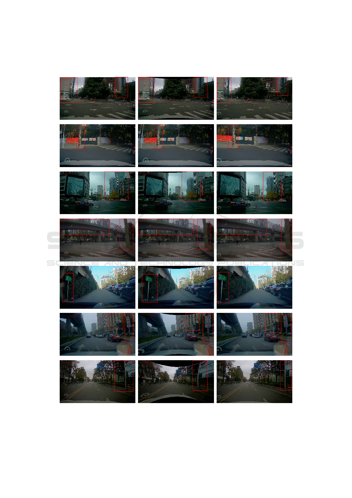
We provide additional qualitative results on the cali-
bration of the D
2
-City dataset. Here, we don’t show
the results from (Chawla et al., 2020a) because it re-
quires corresponding GPS headings that are missing
for this dataset. Note that (Santana-Cedr
´
es et al.,
2017) is run with their default parameters. As shown
in Fig. 8, sometimes (Santana-Cedr
´
es et al., 2017)
fails to completely undistort the structures, while our
method performs consistently across a variety of real-
world situations. Note that the average estimated fo-
cal length for D
2
-City cameras is ≈ 1400 px, different
from the range of values for the KITTI and the Oxford
Robotcar datasets.
Practical Auto-calibration for Spatial Scene-understanding from Crowdsourced Dashcamera Videos
879

Input
Santana et al. 2017
Ours
D
2
City
Figure 8: Additional qualitative comparison of camera auto-calibration on the D
2
-city dataset.
VISAPP 2021 - 16th International Conference on Computer Vision Theory and Applications
880