Intel RealSense SR305, D415 and L515: Experimental Evaluation and

Comparison of Depth Estimation

Francisco Lourenc¸o

and Helder Araujo

Institute of Systems and Robotics, Department of Elec. and Comp. Eng.,University of Coimbra, Coimbra, Portugal

Keywords:

RGB-D Cameras, Experimental Evaluation, Experimental Comparison.

Abstract:

In the last few years, Intel has launched several low-cost RGB-D cameras. Three of these cameras are the

SR305, the L415, and the L515. These three cameras are based on different operating principles. The SR305

is based on structured light projection, the D415 is based on stereo based also using the projection of random

dots, and the L515 is based on LIDAR. In addition, they all provide RGB images. In this paper, we perform

an experimental analysis and comparison of the depth estimation by the three cameras.

1 INTRODUCTION

Consumer-level RGB-D cameras are affordable,

small, and portable. These are some of the main fea-

tures that make these types of sensors very suitable

tools for research and industrial applications, rang-

ing from practical applications such as 3D recon-

struction, 6D pose estimation, augmented reality, and

many more (Zollh

ofer et al., 2018). For many applica-

tions, it is essential to know how accurate and precise

an RGB-D camera is, to understand which sensor best

suits the speciﬁc application (Cao et al., 2018). This

paper aims to compare three models of RGB-D cam-

eras from Intel, which can be useful for many users

and applications.

The sensors are the RealSense SR305, D415, and

L515. Each sensor uses different methods to calculate

depth. The SR305 uses coded light, where a known

pattern is projected into the scene and, by evaluat-

ing how this pattern deforms, depth information is

computed. The D415 uses stereo vision technology,

capturing the scene with two imagers and, by com-

puting the disparity on the two images, depth can be

retrieved. Finally, the L515 that measures time-of-

ﬂight, i.e., this sensor calculates depth by measuring

the delay between light emission and light reception.

Several different approaches can be used to evalu-

ate depth sensors (P.Rosin et al., 2019),(Fossati et al.,

2013). In this case, we focused on accuracy and re-

peatability. For this purpose, the cameras were eval-

https://orcid.org/0000-0001-7081-5641

https://orcid.org/0000-0002-9544-424X

uated using depth images of 3D planes at several dis-

tances, but whose ground truth position and orien-

tation were not used as we don’t know them. Ac-

curacy was measured in terms of point-to-plane dis-

tance, and precision was measured as the repeatability

of 3D model reconstruction, i.e., the standard devia-

tion of the parameters of the estimated 3D model (in

this case, a 3D plane). We also calculated the aver-

age number of depth points per image where the cam-

eras failed to calculate depth (and their standard de-

viation), and the number of outliers per image (points

for which the depth was outside an interval). More-

over, we employ directional statistics (Kanti V. Mar-

dia, 1999) on the planes’ normal vectors to better il-

lustrate how these models variate.

2 RELATED WORK

Depth cameras and RGB-D cameras have been an-

alyzed and compared in many different ways. In

(Halmetschlager-Funek et al., 2019) several param-

eters of ten depth cameras were experimentally an-

alyzed and compared. In addition to that, an anal-

ysis of the cameras’ response to different materials,

noise characteristics, and precision were also evalu-

ated. A comparative study on structured light and

time-of-ﬂight based Kinect cameras is done in (Sar-

bolandi et al., 2015). In (Chiu et al., 2019) depth cam-

eras were compared considering medical applications

and their speciﬁc requirements. Another comparison

for medical applications is performed in (Siena et al.,

362

Lourenço, F. and Araujo, H.

Intel RealSense SR305, D415 and L515: Experimental Evaluation and Comparison of Depth Estimation.

DOI: 10.5220/0010254203620369

In Proceedings of the 16th International Joint Conference on Computer Vision, Imaging and Computer Graphics Theory and Applications (VISIGRAPP 2021) - Volume 4: VISAPP, pages

362-369

ISBN: 978-989-758-488-6

2018). A comparison for agricultural applications is

performed in (Vit et al., 2018). Analysis for robotic

applications is performed in (Jing et al., 2017). In

(Anxionnat et al., 2018) several RGB-D sensors are

analyzed and compared based on controlled displace-

ments, with precision and accuracy evaluations.

3 METHODOLOGY

3.1 Materials

As aforementioned, the sensors used in this evalu-

ation employ different depth estimation principles,

which yields information about the sensor’s perfor-

mance and how these technologies compare to each

other (for the speciﬁc criteria used).

The SR305 uses coded light, the D415 uses stereo

vision, and the L515 uses LIDAR. The camera spec-

iﬁcations are represented on table 1. The three cam-

eras were mounted on the standard tripod.

To ensure constant illumination conditions, a LED

ring (eff, 2020) was used as the only room illumina-

tion source.

Table 1: Sensors resolution (px*px) and range (m).

Sensor SR305 D415 L515

Depth 640x480 1280x720 1024x768

Color 1920x1080 1920x1080 1920x1080

Range [0.2 1.5] [0.3 10] [0.25 9]

Note that the values on table 1 are upper bounds,

meaning that the speciﬁcations may vary for different

sensors’ conﬁgurations. It is also important to men-

tion that the D415 range may vary with the light con-

ditions.

3.2 Experimental Setup

Each camera was mounted on a tripod and placed at

a distance d of a wall. The wall is white and covers

all the ﬁeld of view of the cameras. The optical axes

of the sensors are approximately perpendicular to the

wall. Placed above the camera is the light source,

above described. The light source points to the wall

in the same direction as the camera. For practical rea-

sons, the light source is slightly behind the camera so

that the camera does not interfere with the light. A

laptop is placed behind the camera where the camera

software is executed and where the images are stored.

All the experiments took place at night, avoiding any

unwanted daylight. Hence, the room’s light was kept

constant between experiments and always sourced by

the same element.

The camera, light source, and laptop were placed

on top of a structure. We wanted everything to be

high relative to the ground to ensure that the sensors

captured neither ﬂoor nor ceiling. For each distance

at which the cameras were placed, 100 images were

acquired. The distances for which both D415 and

L515 were tested are 0.5m, 0.75m, 1m, 1.25m, 1.5m,

1.75m, 2m, 2.5m, 3m, and 3.5m. The furthest dis-

tance was the maximum distance for which neither

ﬂoor nor ceiling appeared on the images. The SR305

was tested at 0.3m, 0.4m, 0.5m, 0.75m, 1m, 1.25m,

and 1.5m. In this case, the furthest distance is the

maximum speciﬁed range for the SR305 sensor.

The experiments started at the closest distance.

The sensors were switched right after the other se-

quentially. After all the images were obtained at that

distance, all the structure was moved away from the

wall by the aforementioned intervals. The structure

moved approximately perpendicularly to the wall.

For the D415 and the L515 sensors, we used cus-

tom conﬁgurations. For the SR305 we used the de-

fault conﬁguration. These conﬁgurations were the

same as those of table 1.

3.3 Software

To deal with the sensors, the Intel RealSense SDK

2.0 was used. The Intel RealSense Viewer applica-

tion was used to check the sensors’ behavior right be-

fore each execution, to check for the direction of the

optical axis and distance. All the other tasks were

executed using custom code and the librealsense2 li-

brary. These tasks include both image acquisition and

storing, camera conﬁguration, and point cloud gen-

eration. This part of the work was executed using

Ubuntu. All the statistical evaluation was performed

in MatLab, on Windows 10.

3.4 Experimental Evaluation

3.4.1 Performance

The performance of the sensors was measured in two

ways. First, we calculated the average number of

points for which the sensor failed to measure depth

and the standard deviation of the same number of

points. Then we do the same for outliers.

Whenever the Intel RealSense SDK 2.0 and cam-

era fail to measure the depth at some point, the corre-

sponding depth is deﬁned as zero. Hence, all we do

here is to count pixels in the depth image with a depth

equal to zero.

Depth values also contain outliers. Outliers can be

deﬁned in several ways. In this case, we considered

Intel RealSense SR305, D415 and L515: Experimental Evaluation and Comparison of Depth Estimation

363

as an outlier every point with a depth value differing

10cm from the expected distance, given the speciﬁc

geometric conﬁguration and setup.

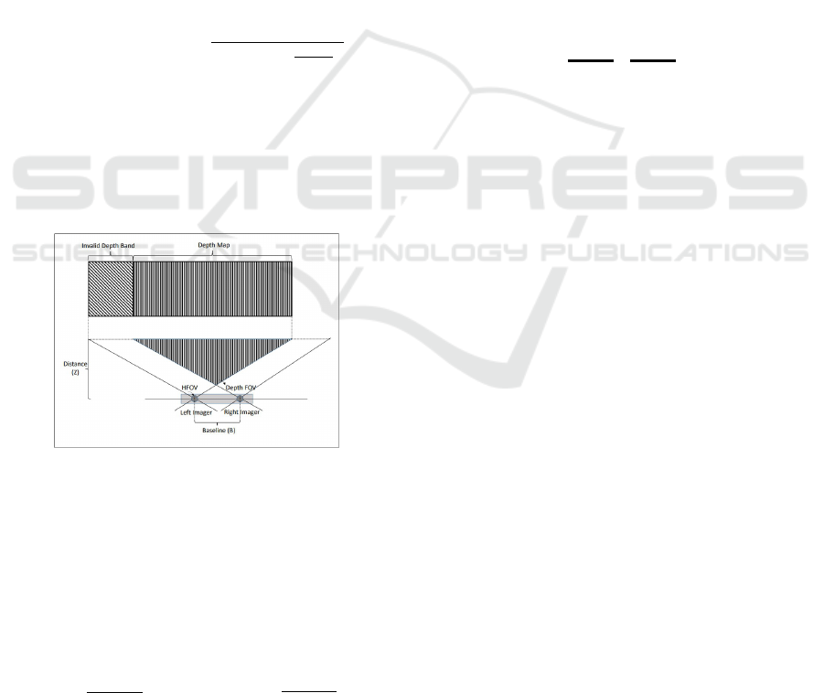
As described in the Intel RealSense D415 prod-

uct DataSheet (D41, 2020), the D415 sensor has an

invalid depth band, which is a region in the depth im-

age for which depth cannot be computed.

The coordinate system of the left camera is used as

the reference coordinate system for the stereo camera.

The left and right cameras have the same ﬁeld of view.

However, due to their relative displacement, there is

an area in the left image for which it is impossible to

compute disparities since the corresponding 3D vol-

ume is not visible in the right camera. It results in a

non-overlap region of the left and right cameras for

which it is impossible to measure depth. This region

appears in the image’s leftmost area and is illustrated

in ﬁgure 1. The total number of pixels in the invalid

depth band can be calculated in pixels as follows:

InvalidDepthBand =

V RES ∗ HRES ∗ B

2 ∗ Z ∗tan(

HF OV

)

(1)

Where V RES and HRES stand for vertical and hori-

zontal resolution respectively (720px and 1280px), B

is the baseline → 55mm, Z is the distance of scene

from the depth module → d and HFOV is the hori-

zontal ﬁeld of view → 64

◦

Bearing that in mind, the pixels in the invalid

depth band were ignored in our calculations.

Figure 1: Invalid Depth Band.

3.4.2 Plane Fitting

Point clouds were ﬁrst obtained using the depth data,

the image pixel coordinates, and the camera intrinsics.

This is possible because we have depth information,

letting the coordinate z be equal to the measured depth

at that point, i.e., z = d

the following equations can

be applied:

x = z ∗

u − pp

(2)

y = z ∗

v − pp

(3)

Where (u, v) are the pixel coordinates, (pp

, pp

)

are the coordinates of the principal point, f

and f

are the focal lengths in pixel units.

The point clouds correspond to a wall. Thus it is

possible to ﬁt a plane to the data.

Since we handle ourselves the outliers, we per-

formed the plane equation’s estimation using standard

least-squares regression, employing the singular value

decomposition, instead of robust approaches such as

RANSAC.

The model we want to be regressed to the point

clouds is the general form of the plane equation:

x ∗ n

+ y ∗ n

+ z ∗ n

− d = 0 (4)

Where (n

) stands for the unit normal, and

d stands for distance from the plane to the origin.

If we now build a n ∗ 4 matrix from the point

clouds with n points, which we will denote as matrix

P. We can rewrite equation 4:

0 =







−1

| {z }

−1



















(5)

By computing the singular value decomposition

on matrix P as:

P = U ∗ Σ ∗V

(6)

We can now use the values of the column of ma-

trix V that corresponds to the smallest eigenvalue in

matrix Σ, as the parameters n

∗

and d

∗

of the

plane that ﬁt that point cloud. Then, we normalize

the plane’s normal vector, which will become handy

in further calculations and recover the true distance in

meters of the plane from the sensor.

3.4.3 Accuracy

For the accuracy analysis, we compute the point-to-

plane distance. For each point of the point cloud, we

use the ﬁtted plane equation to compute the errors,

i.e., the point-to-plane distance. We then calculate the

average root mean square error for each set of 100

images as an accuracy measurement. For the sake of

comparison, we perform this computation for two dif-

ferent threshold values for outlier rejection (±10cm

and ±35cm), another one where we use all points with

the measured depth.

3.4.4 Precision

In this work, precision is measured as per image plane

consistency, i.e., how the plane model changes in be-

tween images of the same sensor at the same distance.

As neither the scene nor the sensor change while tak-

ing the pictures, we could expect the models to be

the exact same if we had an ideal sensor. Thus, by

VISAPP 2021 - 16th International Conference on Computer Vision Theory and Applications

364

measuring the standard deviation of the plane model

parameters in between images, we might be able to

better understand how consistent the sensors are with

their measurements and how this consistency varies

with the distance.

Additionally, we also transform the plane’s nor-

mal vector into spherical coordinates, where we can

perform analysis of directional statistics as all the nor-

mals are distributed on a spherical surface. Speciﬁ-

cally, the circular mean and standard deviation of an-

gles θ and φ, and the spherical variance of the normal

vectors. Since ~n

is unitary, its norm ρ is 1.

Let θ and φ be the azimuth and altitude angles of

= arctan

(7)

= arctan

+ n

(8)

As in (Kanti V. Mardia, 1999), the circular mean

of the angles above can be computed as follows:

θ = arctan

∑

i=1

sinθ

∑

i=1

cosθ

(9)

φ = arctan

∑

i=1

sinφ

∑

i=1

cosφ

(10)

Now, to show how the spherical variance is com-

puted, we need to introduce vector~n, which is the vec-

tor whose components are the mean of each compo-

nent of ~n. If we now compute the norm of ~n and call

it R, the spherical variance is calculated as follows:

V = 1 − R (11)

4 RESULTS

4.1 Performance Analysis

In tables 2, 3 (In Appendix) and ﬁgure 2, we show

the results for the average number of failed points

and the standard deviation of the number of failed

points per image (points where the sensor could not

compute depth). As it can be veriﬁed, the L515 sen-

sor outperforms both D415 and SR305. This sensor

not only showed to be capable of estimating more

depth data relative to its resolution, but the results also

show that that number (of failed points) remains al-

most constant up until 2 meters of distance. This can

be explained by the fact that this sensor uses LIDAR

technology, which is more robust than the stereo vi-

sion and coded light approaches since LIDAR directly

computes depth.

On the other hand, the D415 sensor shows much

better results than the SR305.

A relevant detail of this performance measurement

is that the standard deviation of the number of failed

depth points for the D415 is not strongly dependent

with the distance, whereas that does not seem to be

the case for the L515.

Tables 4, 5 (In Appendix) and ﬁgure 3 include the

results for the number of outliers. Just as it happened

in terms of the average number of failed depth points,

the data for the D415 camera show an increase in the

average number of outliers as the distance increases.

On the other hand, the number of outliers for the

SR305 seems to decrease with increasing distances.

These results are quite different from those presented

in table 2 (In Appendix). The main reason for these

results is probably because the SR305 camera is es-

timating a relatively small number of depth points at

higher distances, therefore decreasing the probability

of outlier occurrences.

To better illustrate this, we show in ﬁgure 4 a sam-

ple image taken with the SR305 sensor at 1.5 meters

of distance, where it is notorious the small amount of

points for which this sensor is measuring depth (the

dark region represents points where the depth was not

computed).

On the other hand, for the case of the L515, the

number of outliers is essentially independent of the

distance. Even though there is some ﬂuctuation in the

numbers, the variation is relatively small. Consider-

ing the standard deviation of the number of outliers

per image obtained with the L515 at 0.75, 1.5, and

1.75 meters, we can see that it is zero, meaning that

the total number of outliers per image stayed constant

over the 100 images. This led us to determine the

pixels where L515 generated outliers. We found out

that the miscalculated points always correspond to the

same pixels from the image’s leftmost column. We

believe that this may be happening to an issue with

the camera used in the experiments, which requires

further investigation.

4.2 Accuracy Analysis

The results of the accuracy study are represented on

table 6 (In Appendix) and in ﬁgure 5, where we plot

the point-to-plane RMSE distances for the three cam-

eras, taking into account only points whose distances

from the expected distance are within 10cm.

Again, the sensor that achieves the best results is

the L515. It not only has the lowest average root mean

Intel RealSense SR305, D415 and L515: Experimental Evaluation and Comparison of Depth Estimation

365

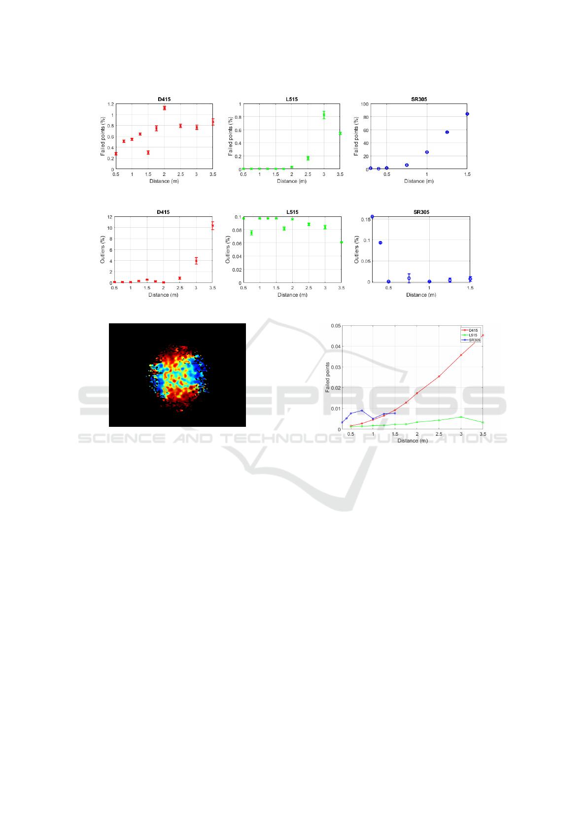
Figure 2: Failed Points - D415 vs L515 vs SR305.

Figure 3: Outliers - D415 vs L515 vs SR305.

Figure 4: SR305 depth image at 1,5m.

square error per image, but it also shows to be the

least sensitive to distance. It should be mentioned that

the image acquisition conditions for the L515 were

close to being optimal since the images were acquired

indoors, without daylight illumination.

In the case of camera D415, its RMSE follows a

smooth increasing pattern as it goes further from the

wall. On the other hand, the RMSE for the SR305

camera does not vary as smoothly with distance. The

RMSE values for this sensor increase until 0.75m and

then start to decrease until 1m. In fact, 1 meter is

the distance for which the SR305 is optimized (SR3,

2020), therefore one should expect this sensor to work

better within this range.

4.3 Precision Analysis

The results show that the camera L515 is signiﬁcantly

more consistent than the other sensors. The results

from tables 7 and 8 (In Appendix), show L515 to be

more precise in terms of 3D estimation. It is notice-

able how this sensor seems to be very consistent be-

tween pictures and for different distances.

Figure 5: Point-To-Plane RMSE D415 vs L515 vs SR305 -

±10cm.

In table 8 (In Appendix) we show the directional

statistics results. The values for the angle θ frequently

change in a non-systematic way. This happens be-

cause, as φ gets closer to 90

◦

, the components n

and

of the normal vector get closer to zero, which will

lead to large variations of the angle θ. For this reason,

we omit the azimuth calculations.

The spherical variation behaves just as expected,

showing again that the L515 sensor is the most sta-

ble and that the measurements from the other two are

more distance sensitive.

For ease of comprehension of our precision re-

sults, we plot on ﬁgures 6 and 7 the standard devia-

tion of parameter d of the plane for all cameras at all

distances, and also the spherical variation.

VISAPP 2021 - 16th International Conference on Computer Vision Theory and Applications

366

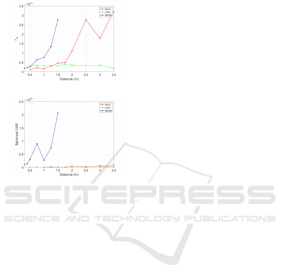
Figure 6: Parameter d standard deviation.

Figure 7: Spherical Variation.

5 CONCLUSION

In this paper, we described a set of experiments

performed to compare the depth estimation perfor-

mance of three RGB-D cameras from Intel, namely

the SR305, the D415, and the L515. In general, the re-

sults show that the L515 is more accurate and precise

than the other two while also providing more stable

and consistent measurements in the speciﬁc environ-

mental conditions of the experiments (indoors with

controlled and stable illumination).

ACKNOWLEDGEMENTS

This work was partially supported by Project COM-

MANDIA SOE2/P1/F0638, from the Interreg Sudoe

Programme, European Regional Development Fund

(ERDF), and by the Portuguese Government FCT,

project no. 006906, reference UID/EEA/00048/2013.

REFERENCES

(2020). Conﬁgurable and powerful ring lights for machine

vision. https://www.efﬁlux.com/en/products/ring/efﬁ-

ring. (Acessed: 05-10-2020).

(2020). Intel

 realsense

d400 series product fam-

ily. https://www.intelrealsense.com/depth-camera-

d415/. (Acessed: 01-10-2020).

(2020). Intel

 realsense

depth camera sr305.

https://www.intelrealsense.com/depth-camera-sr305/.

(Acessed: 02-10-2020).

Anxionnat, Adrien, Voros, Sandrine, Troccaz, and Jocelyne

(2018). Comparative study of RGB-D sensors based

on controlled displacements of a ground-truth model

1. In 2018 15th International Conference on Con-

trol, Automation, Robotics and Vision, ICARCV 2018,

pages 125–128.

Cao, Yan-Pei, Kobbelt, Leif, Hu, and Shi-Min (2018). Real-

time High-accuracy 3D Reconstruction with Con-

sumer RGB-D Cameras. ACM Transactions on

Graphics, 1(1).

Chiu, C.-Y., Thelwell, M., Senior, T., Choppin, S., Hart,

J., and Wheat, J. (2019). Comparison of depth cam-

eras for three-dimensional reconstruction in medicine.

Journal of Engineering in Medicine, 233(9).

Fossati, A., Gall, J., Grabner, H., Ren, X., and Konolige, K.,

editors (2013). Consumer Depth Cameras for Com-

puter Vision. Springer.

Halmetschlager-Funek, G., Suchi, M., Kampel, M., and

Vincze, M. (2019). An empirical evaluation of ten

depth cameras: Bias, precision, lateral noise, different

lighting conditions and materials, and multiple sensor

setups in indoor environments. IEEE Robotics and

Automation Magazine, 26(1):67–77.

Jing, C., Potgiete, J., Noble, F., and Wang, R. (2017). A

comparison and analysis of rgb-d cameras’depth per-

formance for robotics application. In Proc. of the

Int- Conf. on on Mechatronics and Machine Vision in

Practice.

Kanti V. Mardia, P. E. J. (1999). Directional Statistics. Wi-

ley Series in Probability and Statistics. John Wiley &

Sons, Inc., Hoboken, NJ, USA, 2nd edition.

P.Rosin, Lai, Y.-K., L.Shao, and Liu, Y., editors (2019).

RGB-D Image Analysis and Processing. Springer.

Sarbolandi, H., Leﬂoch, D., and Kolb, A. (2015). Kinect

range sensing: Structured-light versus time-of-ﬂight

kinect. Computer Vision and Image Understanding,

139:1 – 20.

Siena, F. L., Byrom, B., Watts, P., and Breedon, P. (2018).

Utilising the Intel RealSense Camera for Measuring

Health Outcomes in Clinical Research. Journal of

Medical Systems, 42(3):1–10.

Vit, Adar, Shani, and Guy (2018). Comparing RGB-D sen-

sors for close range outdoor agricultural phenotyping.

Sensors (Switzerland), 18(12):1–17.

Zollh

ofer, Michael, Stotko, Patrick, G

orlitz, Andreas,

Theobalt, Christian, Nießner, M., Klein, R., and Kolb,

A. (2018). State of the art on 3D reconstruction

with RGB-D cameras. Computer Graphics Forum,

37(2):625–652.

Intel RealSense SR305, D415 and L515: Experimental Evaluation and Comparison of Depth Estimation

367

APPENDIX

Table 2: Average of failed points ratio per image by distance

in meters.

d D415 L515 d SR305

0.5 0.2801% 0.0020% 0.3 1.3967%

0.75 0.5099% 0.0001% 0.4 0.6062%

1 0.5414% 0.0023% 0.5 1.6930%

1.25 0.6415% 0.0001% 0.75 6.0734%

1.5 0.3025% 0.0014% 1 25.8181%

1.75 0.7472% 0.0017% 1.25 56.3898%

2 1.1202% 0.0320% 1.5 84.2698%

2.5 0.7945% 0.1648% — —

3 0.7660% 0.8263% — —

3.5 0.8644% 0.5456% — —

Table 3: Standard deviation of failed points ratio per image

by distance in meters.

d D415 L515 d SR305

0.5 0.0248% 0.0023% 0.3 0.0397%

0.75 0.0224% 0.0003% 0.4 0.0198%

1 0.0195% 0.0050% 0.5 0.0415%

1.25 0.0211% 0.0004% 0.75 0.0783%

1.5 0.0329% 0.0033% 1 0.1282%

1.75 0.0458% 0.0025% 1.25 0.1886%

2 0.0319% 0.0100% 1.5 0.2714%

2.5 0.0335% 0.0278% — —

3 0.0378% 0.0570% — —

3.5 0.0585% 0.0155% — —

Table 4: Average of outliers ±10cm ratio per image by dis-

tance in meters.

d D415 L515 d SR305

0.5 0.1141% 0.0968% 0.3 0.1560%

0.75 0.1112% 0.0753% 0.4 0.0933%

1 0.0667% 0.0968% 0.5 0%

1.25 0.2809% 0.0968% 0.75 0.0081%

1.5 0.5387% 0.0968% 1 3.9062%

1.75 0.2568% 0.0813% 1.25 0.0032%

2 0.0558% 0.0957% 1.5 0.0063%

2.5 0.8361% 0.0882% — —

3 3.9436% 0.0839% — —

3.5 10.3307% 0.0609% — —

Table 5: Standard deviation of outliers ±10cm ratio per im-

age by distance in meters.

d D415 L515 d SR305

0.5 0.0209% 0% 0.3 0.0004%

0.75 0.0193% 0.0034% 0.4 0.0018%

1 0.0139% 1.2715% 0.5 0%

1.25 0.0226% 0% 0.75 0.0105%

1.5 0.0380% 0% 1 0.0003%

1.75 0.0431% 0.0025% 1.25 0.0046%

2 0.0168% 0.0008% 1.5 0.0057%

2.5 0.1892% 0.0018% — —

3 0.5601% 0.0027% — —

3.5 0.7226% 0.0001% — —

Table 6: Sensors’ accuracy in terms of average root mean

square point-to-plane distance error per image.

Cam

dist

±10cm ±35cm All Points

D415

0,5m

0,002 0,004 0,122

D415

0,75m

0,003 0,003 0,087

D415

0,005 0,005 0,079

D415

1,25m

0,007 0,007 0,037

D415

1,5m

0,009 0,009 0,139

D415

1,75m

0,013 0,013 0,293

D415

0,017 0,017 0,093

D415

2,5m

0,025 0,027 0,036

D415

0,036 0,042 0,069

D415

3,5m

0,045 0,063 0,065

L515

0,5m

0,001 0,001 134,853

L515

0,75m

0,001 0,001 202,285

L515

0,001 0,001 150,913

L515

1,25m

0,002 0,002 7,556

L515

1,5m

0,002 0,002 14,588

L515

1,75m

0,002 0,002 22,389

L515

0,002 0,002 15,542

L515

2,5m

0,003 0,003 14,865

L515

0,004 0,004 25,025

L515

3,5m

0,006 0,006 13,835

SR305

0,3m

0,003 0,036 113,994

SR305

0,4m

0,005 0,005 114,889

SR305

0,5m

0,008 0,008 0,008

SR305

0,75m

0,009 0,009 0,009

SR305

0,005 0,005 0,006

SR305

1,25m

0,007 0,007 0,008

SR305

1,5m

0,008 0,008 0,011

VISAPP 2021 - 16th International Conference on Computer Vision Theory and Applications

368

Table 7: Camera precision in terms of plane modelling consistency.

Cam

dist

d σ

D415

0,5m

3,9E-03 2,5E-04 4,1E-03 2,1E-04 1,0E+00 1,5E-06 -5,0E-01 1,1E-04

D415

0,75m

3,7E-03 3,0E-04 -8,8E-03 2,0E-04 1,0E+00 1,5E-06 -7,5E-01 2,2E-04

D415

1,7E-02 7,2E-04 -1,3E-03 2,6E-04 1,0E+00 1,3E-05 -1,0E+00 1,6E-04

D415

1,25m

1,4E-02 1,6E-03 -2,7E-03 3,6E-04 1,0E+00 1,8E-05 -1,3E+00 3,1E-04

D415

1,5m

1,8E-02 8,7E-04 3,0E-03 4,3E-04 1,0E+00 1,6E-05 -1,5E+00 4,6E-04

D415

1,75m

2,2E-02 8,5E-04 3,4E-04 5,8E-04 1,0E+00 1,8E-05 -1,8E+00 4,9E-04

D415

1,3E-02 2,9E-03 2,4E-03 8,6E-04 1,0E+00 2,9E-05 -2,0E+00 1,1E-03

D415

2,5m

1,0E-02 1,5E-03 -3,2E-03 9,3E-04 1,0E+00 1,4E-05 -2,5E+00 2,8E-03

D415

1,4E-02 3,2E-03 -5,8E-04 1,1E-03 1,0E+00 3,3E-05 -3,0E+00 1,8E-03

D415

3,5m

6,6E-03 1,8E-03 1,8E-03 1,3E-03 1,0E+00 1,2E-05 -3,5E+00 3,2E-03

L515

0,5m

-4,6E-05 6,1E-04 -2,9E-03 2,3E-04 1,0E+00 7,9E-07 -5,0E-01 3,5E-04

L515

0,75m

1,8E-03 4,6E-04 -2,7E-03 1,6E-04 1,0E+00 7,1E-07 -7,5E-01 3,3E-04

L515

-1,9E-03 6,1E-04 -5,7E-03 1,5E-04 1,0E+00 1,9E-06 -1,0E+00 3,5E-04

L515

1,25m

-6,8E-06 3,1E-04 2,1E-03 7,6E-05 1,0E+00 1,9E-07 -1,3E+00 3,1E-04

L515

1,5m

-3,1E-03 5,2E-04 -9,2E-04 1,9E-04 1,0E+00 1,7E-06 -1,5E+00 3,3E-04

L515

1,75m

1,8E-03 3,3E-04 3,1E-04 1,0E-04 1,0E+00 6,2E-07 -1,8E+00 3,1E-04

L515

-8,0E-04 4,5E-04 -5,1E-04 1,7E-04 1,0E+00 4,4E-07 -2,0E+00 3,9E-04

L515

2,5m

3,2E-04 3,5E-04 -8,7E-04 1,4E-04 1,0E+00 1,7E-07 -2,5E+00 3,5E-04

L515

-2,1E-03 3,3E-04 -3,9E-03 1,5E-04 1,0E+00 1,1E-06 -3,0E+00 3,3E-04

L515

3,5m

1,7E-03 4,0E-04 -6,8E-03 8,3E-05 1,0E+00 7,7E-07 -3,5E+00 3,5E-04

SR305

0,3m

4,4E-03 4,6E-03 -5,6E-03 1,0E-04 1,0E+00 2,7E-05 -3,0E-01 1,8E-04

SR305

0,4m

7,7E-03 5,2E-03 -8,2E-04 8,7E-05 1,0E+00 6,2E-05 -4,0E-01 2,3E-04

SR305

0,5m

1,7E-02 7,8E-03 5,2E-03 1,2E-04 1,0E+00 1,6E-04 -5,0E-01 2,7E-04

SR305

0,75m

-1,7E-02 1,3E-02 -1,3E-04 2,8E-04 1,0E+00 2,6E-04 -7,5E-01 6,3E-04

SR305

-1,7E-02 7,3E-03 6,6E-03 1,8E-04 1,0E+00 1,0E-04 -1,0E+00 7,7E-04

SR305

1,25m

-2,7E-02 1,2E-02 -2,3E-03 5,0E-04 1,0E+00 2,6E-04 -1,3E+00 1,3E-03

SR305

1,5m

-2,3E-02 2,0E-02 -2,9E-03 1,1E-03 1,0E+00 5,8E-04 -1,5E+00 2,8E-03

Table 8: Camera precision in terms of plane normal vector angles standard deviation and spherical variance.

Cam

dist

φ σ

V C am

dist

φ σ

D415

0,5m

9,0E+01 1,5E-02 5,3E-08 L515

1,5m

9,0E+01 3,1E-02 1,5E-07

D415

0,75m

8,9E+01 9,2E-03 6,5E-08 L515

1,75m

9,0E+01 1,9E-02 5,9E-08

D415

8,9E+01 4,1E-02 2,9E-07 L515

9,0E+01 2,4E-02 1,2E-07

D415

1,25m

8,9E+01 8,5E-02 1,3E-06 L515

2,5m

9,0E+01 8,6E-03 7,3E-08

D415

1,5m

8,9E+01 4,9E-02 4,7E-07 L515

9,0E+01 1,4E-02 6,5E-08

D415

1,75m

8,9E+01 4,9E-02 5,3E-07 L515

3,5m

9,0E+01 6,2E-03 8,3E-08

D415

8,9E+01 1,6E-01 4,6E-06 SR305

0,3m

9,0E+01 1,5E-01 1,1E-05

D415

2,5m

8,9E+01 7,9E-02 1,6E-06 SR305

0,4m

9,0E+01 3,0E-01 1,4E-05

D415

8,9E+01 1,7E-01 5,6E-06 SR305

0,5m

8,9E+01 4,2E-01 3,1E-05

D415

3,5m

9,0E+01 1,0E-01 2,5E-06 SR305

0,75m

8,9E+01 7,0E-01 9,0E-05

L515

0,5m

9,0E+01 1,4E-02 2,1E-07 SR305

8,9E+01 3,2E-01 2,7E-05

L515

0,75m

9,0E+01 1,2E-02 1,2E-07 SR305

1,25m

8,8E+01 5,6E-01 7,4E-05

L515

9,0E+01 1,8E-02 2,0E-07 SR305

1,5m

8,9E+01 1,0E+00 2,1E-04

L515

1,25m

9,0E+01 4,8E-03 5,2E-08 — — — —

Intel RealSense SR305, D415 and L515: Experimental Evaluation and Comparison of Depth Estimation

369