Supporting Detection of Near and Far Pedestrians in a Collision
Prediction System
Lucas F. S. Cambuim
a
and Edna Barros
b
Center of Informatics, Federal University of Pernambuco - UFPE, Recife, Brazil
Keywords:
Pedestrian Detection, Distance Estimation, Stereo Vision, Trajectory Prediction, Collision Prediction.
Abstract:
This paper proposes a multi-window-based detector to locate pedestrians near and distant. This detector is
introduced in a pedestrian collision prediction (PCP) system. We developed an evaluation strategy for the pro-
posed PCP system based on a synthetic collision database, which allowed us to analyze collision prediction
quality improvements. Results demonstrate that the combination of different window subdetectors outper-
forms individual subdetectors’ accuracy and YOLO-based detector. Once our system achieved a processing
rate of 30 FPS when processing images in HD resolution, results demonstrated an increase in the number of
scenarios that the system could entirely avoid a collision compared to a YOLO-based system.
1 INTRODUCTION
Pedestrians represent more than half of all the global
deaths in transit accidents (Organization, 2018).
Pedestrian collision prediction (PCP) systems are fun-
damental in reducing accidents because they per-
mit efficient and early decision-making (Haas et al.,
2020). Camera-based sensors have been widely
adopted in PCP systems because they provide high-
resolution features that permit PCP systems to under-
stand the pedestrian’s behavior and intention (Haas
et al., 2020).
Given that automobiles are getting faster and
faster, PCP systems capable of predicting pedestri-
ans’ collisions over long distances are desirable. The
higher the speed, the greater the distance to stop the
vehicle. Also, on a wet road, this distance tends to be
longer (Li et al., 2020).
Most of the detectors typically perform sliding
fixed-size window with HOG-based feature extractors
(Dalal and Triggs, 2005). These detectors typically
support 128 × 64 windows and work reasonably well
with large-sized pedestrians near the camera. How-
ever, when the target pedestrians are smaller than 128
× 64 (i.e., more distant), the detector almost always
fails to detect any pedestrian.
Thus, this paper presents a PCP system that com-
bines several trained HOG-based subdetectors with
a
https://orcid.org/0000-0001-5577-7368
b
https://orcid.org/0000-0001-6479-3052
different window sizes to capture pedestrians both
near and far. Also, some significant contributions are
described as follow:
• We propose an approach for distance estima-
tion that deals with bad-fitted bounding boxes in
pedestrian detection and a geometric filtering ap-
proach to reduce false positives
• To evaluate PCP systems, we propose synthetic
collision scenarios involving an occluded pedes-
trian crossing in front of the moving car. These
scenarios represent most accidents and are chal-
lenging because of the need for a fast reaction
from the vehicle.
• Our system achieves an 11% miss rate against
42% of the YOLO-based system in real scenarios,
and our system predicted a collision faster than the
YOLO-based system in 27 out of 35 scenarios.
The paper organization is the following. Section
2 describes some existing vision-based PCP systems
and pedestrian detection approaches. Section 3 de-
scribes the details of the proposed PCP system. Sec-
tion 4 presents an evaluation of the proposed system
and comparatives with related works, and finally, Sec-
tion 5 concludes the paper.
2 RELATED WORKS
Great efforts have been made to the pedestrian detec-
tion task to solve the challenges in developing PCP
Cambuim, L. and Barros, E.
Supporting Detection of Near and Far Pedestrians in a Collision Prediction System.
DOI: 10.5220/0010253706690676
In Proceedings of the 16th International Joint Conference on Computer Vision, Imaging and Computer Graphics Theory and Applications (VISIGRAPP 2021) - Volume 4: VISAPP, pages
669-676
ISBN: 978-989-758-488-6
Copyright
c
 2021 by SCITEPRESS – Science and Technology Publications, Lda. All rights reserved
669

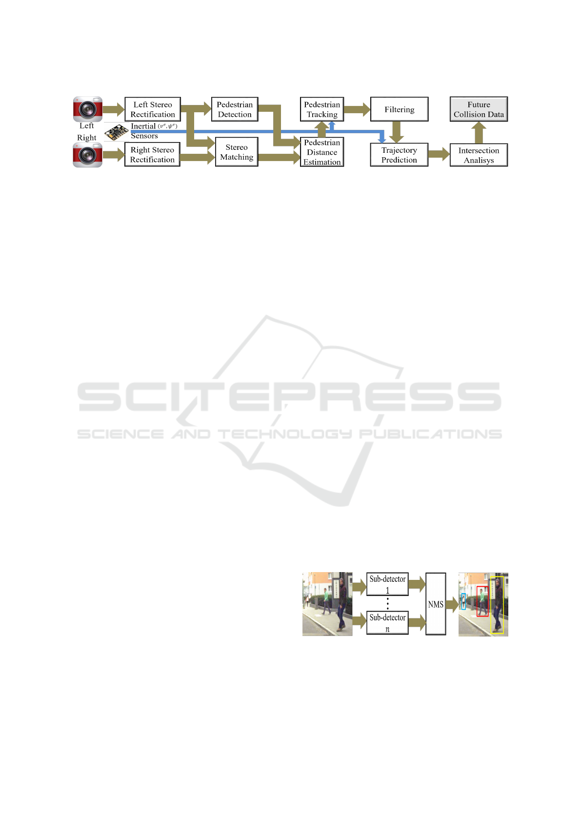
Figure 1: The general architecture of the proposed PCP system.
systems. The histogram of oriented gradient or HOG
descriptor by Dalal and Triggs (Dalal and Triggs,
2005) is perhaps the most well-known feature engi-
neering technique constructed for pedestrian detec-
tion. HOG served as a base for the emergence of
many other techniques (Benenson et al., 2014). HOG
has been employed in the PCP system proposed by
(Keller et al., 2011) with 48 × 96 windows. With
this window size, the authors only detect pedestrians
between 10 and 25 meters. Besides, all the steps’ pro-
cessing performance reaches a rate of 15 FPS, operat-
ing at VGA image resolution (i.e., 640 × 480).
Other pedestrian detectors category is based
on deep convolutional neural networks (CNN)
(Krizhevsky et al., 2012). Many variants of CNN-
based techniques achieved state-of-the-art pedestrian
detection performance, for example, YOLO (You
only look once) (Redmon and Farhadi, 2018). YOLO
can detect pedestrians at various scales and aspect ra-
tio in the image. However, in the specific case of
pedestrians far away, even at high proportions of false
positives, YOLO and other CNN-based detectors still
have too low recall rates.
One way to work around the deficiency of detect-
ing distant people is to process frames with increas-
ing resolutions. However, CNN-based detectors have
a high computational cost that prevents us from ob-
taining efficient processing solutions (Nguyen et al.,
2019). On the other hand, HOG-based approaches
combined with shallow linear classifiers such as SVM
can achieve high processing rates (Helali et al., 2020)
due to their relatively regular and straightforward pro-
cessing. With the implementation of HOGs efficiently
calculating frames at high resolutions, we could ex-
plore multiple windows and small window sizes to
capture pedestrians further and further away.
3 PROPOSED PCP SYSTEM
Figure 1 shows an overview of a PCP system’s pro-
posed architecture. We use a stereo camera system at-
tached to the vehicle to capture stereo frame pairs. Ve-
hicle movement data such as speed (v
e
) and yaw rate
(
˙
ψ
e
) are collected from inertial sensors and aligned
with each frame.
Corrections of radial and tangential distortions
and horizontal alignment are performed in each frame
by the stereo rectification stage (Hartley and Zis-
serman, 2003). The stereo matching step calcu-
lates the disparity map that informs each pixel’s dis-
tance. We adopted the Semi-Global Matching (SGM)
(Hirschmuller, 2008) technique that performs an op-
timization throughout the entire image, producing
more robust and accurate disparity maps for the ur-
ban context. Problems of occlusion and mismatched
disparities are faced by stereo matching approaches
that reduce pedestrian distance estimation accuracy.
We use the L/R check technique (Hirschmuller, 2008)
to find such pixels. The techniques proposed for the
remaining steps are detailed as follows.
3.1 Pedestrian Detection
The pedestrian detection aims to find pedestrians by
bounding boxes. We proposed to this step, an ap-
proach that combines several trained detectors with
different window sizes to capture pedestrians of var-
ious sizes and distances, as shown in Figure 2. Each
subdetector includes an image pyramid technique, a
sliding window, HOG, and a linear SVM. The im-
age pyramid technique with a scale factor of θ
scale
deals with pedestrians with larger dimensions than the
detector window dimension. Parameters ∆
u
and ∆
v
,
from the sliding window, define the shift between de-
tection windows on the axis u and v, respectively, in
the image.
Figure 2: Multi-window-based detector.
Each subdetector returns bounding boxes whose
confidence score is greater than σ
svm
. We perform
a Non-Maximum Suppression (NMS) step to remove
several neighboring predictions from the same pedes-
VISAPP 2021 - 16th International Conference on Computer Vision Theory and Applications
670

trian. Typically, two bounding boxes BB
i
and BB
j
are supposed to correspond to a unique pedestrians
if the overlap defined by Equation 1 is above a thresh-
old θ
nms
= 0.5. We select the highest-scoring bound-
ing box and then remove all the bounding boxes with
enough overlap.
Γ(BB
i
,BB
j
) =
area(BB
i
∩ BB
j
)
area(BB
i
∪ BB
j
)
(1)
To train each pedestrian detector, we have cre-
ated, from a given database with labeled pedestrians,
a set of cropped images containing pedestrians (i.e.,
positive sample) and non-pedestrians (i.e., negative
sample). Firstly, we select positive samples for con-
structing a training set. We permit pedestrians to be
included in the positive sample even if their dimen-
sions are smaller than the subdetector dimension. To
be included, the differences between pedestrian width
and detector width and pedestrian height and detec-
tor height have to be respectively smaller than th
width
and th
height
pixels. Thus, each subdetector can detect
pedestrians with smaller distances than those permit-
ted in its window dimension.
We perform data augmentation applying horizon-
tal mirroring, image rotation, and contrast changing
for each pedestrian location in the left image. When
there exist disparity information and stereo image, we
also collect cutouts from the right image. We ap-
plied a bootstrapping algorithm to increase the nega-
tive sample from an initial small negative sample ob-
tained at random positions. The algorithm collects the
incorrectly classified samples for the first time, adds
these samples to the negative sample set, and retrains
the SVM. The process is repeated several times until
the detection precision achieves the convergence, or
the amount of negative samples equals the amount of
positive sample.
3.2 Distance Estimation
We calculate each pedestrian’s lateral and longitudi-
nal distances in two steps, as shown in Figure 3: (1)
search for the greatest disparity value and (2) average
of the disparity and lateral distance values.
Figure 3: The pedestrian distance estimation approach.
In the first step, we search the greatest valid dis-
parity value in a rectangular region ℵ
k
with a width
equal to the bounding box width and height of 5 pixels
centered in the middle of the bounding box of a given
detected pedestrian k. We called this value disp
k
max
. In
the second step, the final disparity and lateral distance
of the pedestrian are estimated by averaging, respec-
tively, the disparities and lateral distance within the
rectangular region ℵ
k
whose absolute disparity dif-
ference to disp
k
max
is less than a given threshold th
disp
.
We set th
disp
= 2 to guarantee selected disparities only
belong to the pedestrian.
3.3 Pedestrian Tracking
The tracking identifies and labels measurements that
belong to the same pedestrian over several consecu-
tive frames. The measurements are the lateral and lon-
gitudinal distances. A pedestrian movement model is
crucial for the effectiveness of the association of mea-
surements and tracks and trajectory prediction. Thus,
we detail the movement model and then the associa-
tion steps.
3.3.1 Pedestrian Motion Model
The constant velocity (CV) model describes the
pedestrian movement through the state variable x =
(x,z,v
x
,v
z
), where x, z, v
x
, and v
z
describe, respec-
tively, the lateral and longitudinal distances; and
the lateral and longitudinal velocities in the cam-
era space. Following the perspective transformation
model (Hartley and Zisserman, 2003), the relation-
ship between the distance p
c
= (x,y,z) in camera’s
coordinates and the distance p
i
= (u,v,d) in image’s
coordinates is as follows:


u
v
d


=


h
1
(p
c
)
h
2
(p
c
)
h
3
(p
c
)


=



f ·x
z
+ u
0
f ·y
z
+ v
0
b· f
z



, (2)
where the parameters b, f and (u
0
,v
0
) are, respec-
tively, the distance between focal centers, the focal
length, and the principal point of the stereo camera
system. As we consider the pedestrian position is on
the ground plane, so v = 0 and h
2
can be ignored.
To reduce the effect of the measurement noise on
the pedestrian’s velocity estimate, we used the ex-
tended version of Kalman filter (EKF) (Bar-Shalom
et al., 2004), which deals with non-linear functions
like that in Equation 2. The EKF estimates the state
x
k
at time step k from measurement z
k
and previous
state x
k−1
with the dynamical model:
ˆ
x
k
= A
k
x
k−1
+ B
k
s
k−1
+ ω
k−1
, (3)
where the relation between measurement and state is
given by
z
k
= H
k
x
k
+ ν
k
(4)
Supporting Detection of Near and Far Pedestrians in a Collision Prediction System
671

The matrices A
k
and B
k
= I
4×4
are transition ma-
trices for the state x and the control input s, respec-
tively, ω
k−1
and ν
k
are white, zero-mean, uncorre-
lated noise of processes and measurements with co-
variances ω
k−1
∼ N (0, Q) and ν
k
∼ N (0, R). Q is
modeled as discrete white noise acceleration with a
standard deviation of σ
x
and R = diag(σ
2
u
,σ
2
d
) where
σ
u
and σ
d
are, respectively lateral and longitudinal
measurement error. Since the transformation function
h in Equation 2 is non-linear, the matrix H
k
is the Ja-
cobian of h.
The coordinate system origin moves along with
the vehicle. Therefore, to know the accurate pedes-
trian movement, we need to compensate for the vehi-
cle movement when we calculate the evolution from
x
k−1
to x
k
. This compensation is defined by the ma-
trix A
k
and by the vector s
k
described as:
A
k
=

R
M
c
,k
0
2×2
0
2×2
R
M
c
,k

A, (5)
s
k
=

t
M
c
,k
0
2×1

, (6)
where A is the traditional transition matrix of the CV
model, R
M
c
,k
∈ R
2×2
and t
M
c
,k
∈ R
2×1
are respec-
tively rotation and translation matrices at the time t
k
.
These matrices are obtained from the inverse ego-
motion homography matrix M
c
described as:
M
c
= D
−1
M
v
D, (7)
where the matrix D defines the relation in homoge-
neous coordinates between the camera and vehicle co-
ordinate system and M
v
is the inertial motion matrix
in vehicle coordinates (Hartley and Zisserman, 2003).
3.3.2 Tracking Association and Management
Figure 4 shows the steps for associating tracks and
measurements. For each track kept by a tracks list,
we calculate the state prediction by Equation 3. Using
the Euclidean distance, we calculate the dissimilarity
between the predicted tracks and the new measure-
ments. These dissimilarity values are used in the gat-
ing step to exclude unlikely associations whose dis-
tance is greater than a fixed threshold of t
gate
. We set
th
gate
= 2 because the same pedestrian can not be two
meters away between consecutive frames. For the re-
maining associations, we carry out the so-called Hun-
garian method to the global one-to-one association of
tracks and measurements, resulting in a list of tracks
matched with measurements, unmatched tracks, and
unmatched measurements.
The tracks manager uses these lists for updating
the existing tracks list that is initially empty. For each
unmatched measurement, the tracks manager creates
Figure 4: Pedestrian tracking approach.
a new track with the initial state x = (x,z,0,0) where x
and z are respectively the lateral and longitudinal dis-
tances from the measurement. For each track created
i, there is a counter C
i
that counts the frames number
since its last successful association, a counter F
i
that
counts the number of successful associations since its
creation, and a status to indicate whether the track is
confirmed or not. C
i
is incremented during the state
forecasting step and reset when the track i is associ-
ated with some measurement. Tracks that exceed a
predefined maximum age of C
max
= 4 probably have
left the scene and are excluded from the tracks list.
New tracks have temporary status initially. When
F
i
is higher than a fixed value of F
min
= 2, the trace
i turns its status into confirmed. However, if any
temporary track does not match any measurement in
the following frames, it is removed from the tracks
list. For each trace i matched with any measurement,
we performed the measurement update of its internal
state from EKF and incremented F
i
. The trajectory
prediction considers only tracks with confirmed sta-
tus.
3.4 Filtering
We perform two types of filtering when obtaining
measurements of pedestrian locations: temporal and
geometric. Temporal filtering is performed through
the tracking approach. When we consider only con-
firmed, we are applying time filtering. Geometric fil-
tering considers locality restrictions on the track and
restriction of pedestrian dimensions. The following
equation describes the geometric filtering function:
D(h
k
,w
k
, f
k
) =





1, if (1.2 < h
k
< 3.5
∧ w
k
< 2.0 ∧
−h
road
< f
k
< h
road
)
0, otherwise
, (8)
where h
k
and w
k
are, respectively, the height and the
width of the pedestrian, and f
k
is the foot’s height
concerning the camera for the one given pedestrian
k in the camera space. We calculate h
k
, w
k
from the
bounding box’s extreme pixels difference converted
to the camera space, and f
k
from the bounding box’s
VISAPP 2021 - 16th International Conference on Computer Vision Theory and Applications
672

Figure 5: Quality of some detectors when locating pedestrians with distances between 10 and 25 meters (Group 1), above 25
meters (Group 2), and above 10 meters (Group 3). We generated σ
svm
values in the interval of [2.0,0.0[ to obtain these results.
lowest point. The term h
road
in the equation is defined
as the camera’s height relative to the vehicle coordi-
nate system plus a tolerance of 1.2 meters. We con-
sider a valid location if this equation is one.
3.5 Trajectory Prediction
The confirmed tracks’ future trajectories are predicted
by executing EKF state prediction steps without the
measurement update step. In a recursive process, for
each variable
ˆ
x
k
estimated in the time step k, the
next variable
ˆ
x
k+1
is predicted to the next time step
k + 1 using Equation
ˆ
x
k+1
= A
ˆ
x
k
. To find future
collisions, the pedestrian predicted positions need to
be transformed into the vehicle space using Equation
ˆ
X
hom
= D
ˆ
x
hom
, where
ˆ
x
hom
is the location in homo-
geneous coordinates of the predicted position.
X = v
e
(
˙
ψ
e
)
−1
[1 − cos(ψ
e
t
f
)] (9)
Z = v
e
(
˙
ψ
e
)
−1
[sin(ψ
e
t
f
)] (10)
The vehicle’s future trajectory is predicted from cur-
rent measurements of yaw rate
˙
ψ
e
and velocity v
e
.
Moving in the radius of curve r = v
e
·
˙
ψ
e
, the lateral
(X) and longitudinal (Z) position in a future time t
f
is
calculated, respectively by Equations 9 and 10.
3.6 Intersection Analysis
We identify possible collision positions when each
pedestrian’s positions are at the same time in the fu-
ture, touching the front of the vehicle. If a pedes-
trian’s position q at the time-step k, (X
q
k
,Z
q
k
), touches
the line composed by the vehicle’s predicted extreme
points, we mark this position as a collision position.
We repeat this procedure for all pedestrians in all fu-
ture positions.
4 RESULTS
We perform two evaluations: (1) of the pedestrian lo-
cation component and (2) of the collision prediction
component. In the following, we show the database
adopted, the results, and analyses. We also show the
processing performance of the proposed PCP system.
4.1 Database Overview
We used the database (Schneider and Gavrila, 2013)
that provides the ground-truth bounding boxes and
distances from the pedestrian to the vehicle in each
frame for both training and testing samples. This
database consists of 68 samples containing a sequence
of stereo frames and the vehicle velocity and yaw rate.
The image resolution is 1176 × 640 pixels, and the
data capture rate is 16 FPS. The samples also contain
scenarios with the vehicle moving or stopped.
4.2 System Configuration
To demonstrate improvements when detecting both
distant and near pedestrians, we defined two subde-
tectors that will make up our multi-window-based
detector. Subdetector 1 is responsible for detecting
pedestrians above 25 meters away. For comparison,
we define this subdetector with similar parameters to
(Keller et al., 2011). Subdetector 2 is responsible
for detecting pedestrians between 10 and 25 meters
away. Both detectors parameters are defined in Table
1. We highlight the descriptor’s cell dimension has
to be small enough to obtain the entire pedestrian’s
salient features. The process noise parameter σ
x
and
measurement noise parameters σ
u
and σ
d
were de-
fined, according to (Schneider and Gavrila, 2013), re-
spectively as 4.0, 6.15, and 0.32.
Table 1: Subdetectors parameters.
Index
Window
size
1
Cell
size
1
Block
size
1
Bins
1
θ
scale
(∆
u
,∆
v
)
1 48 × 96 4 × 4 2 × 2 9 1.1 (4,4)
2 64 × 128 8 × 8 2 × 2 9 1.1 (8, 8)
1
Parameters from HOG approach.
We use the training set to train each subdetector.
We create positive and negative patches for each de-
Supporting Detection of Near and Far Pedestrians in a Collision Prediction System
673

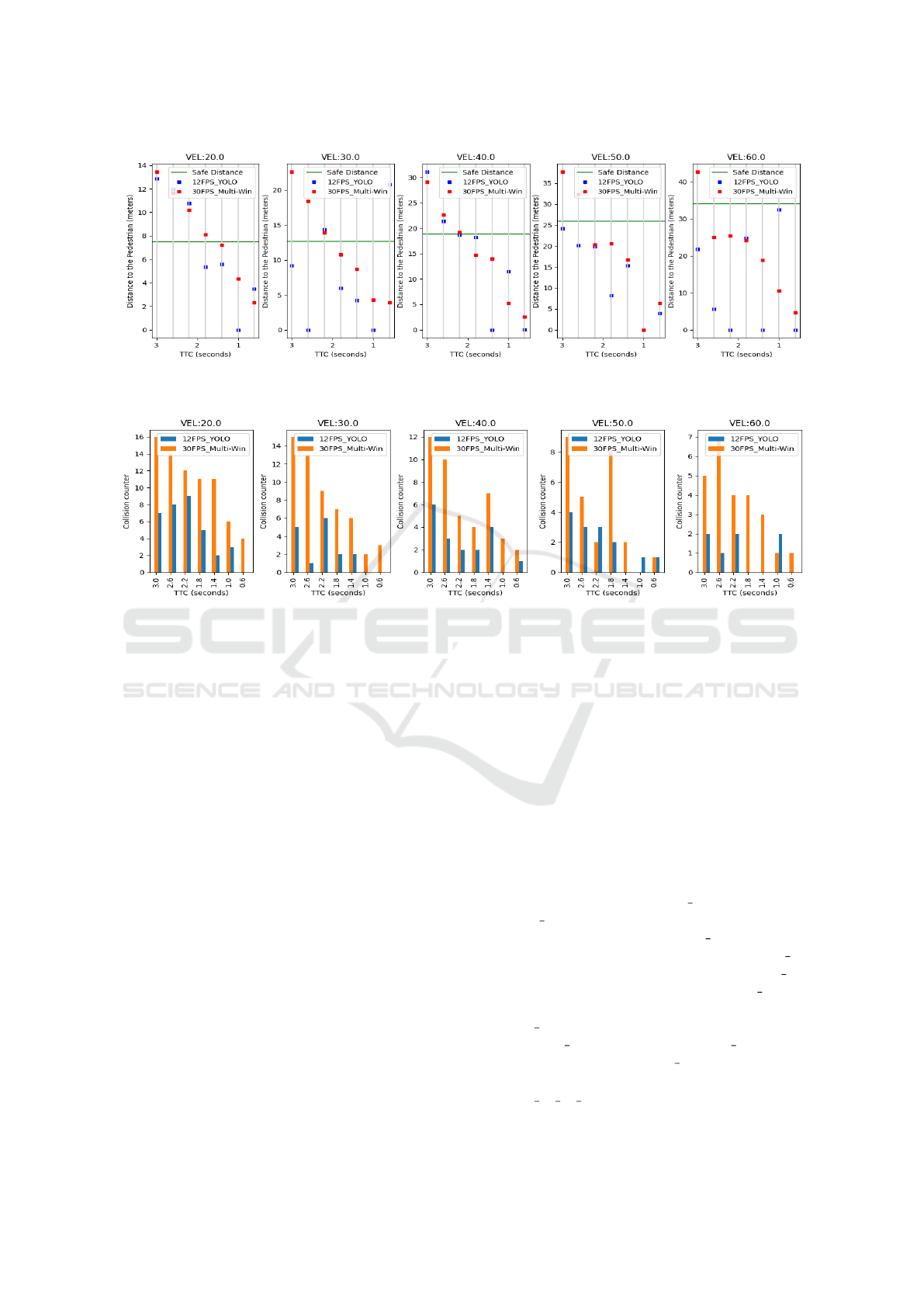
Figure 6: First collision prediction since the pedestrian’s emergence. The comparison was made involving our multi-window
detector (Multi-Win) and the YOLO-based detector.
Figure 7: Amount of collision prediction since the the pedestrian’s emergence. The comparison was made involving our
multi-window detector (Multi-Win) and the YOLO-based detector.
tector following the strategy defined in Section 3.1.
We set th
width
and th
height
as respectively 40 and 20
pixels. The following data augmentation parameters
have been carefully defined to permit the detector ac-
curacy convergence during the training phase.
• Rotation (radian): ±[0.1, 0.15, 0.20, 0.25]
• Scale: +[0.7, 0.75, 0.80, 0.85, 0.90]
• Contrast: +[0.7, 0.8, 1.2, 1.3]
Using this database, it was also possible to obtain
clippings in the right image from the disparity pro-
vided. For each generation of patches, we also per-
form horizontal mirroring. Thus, for subdetector 1,
we had 9,504 positive clippings and 9,504 negative
clippings; for subdetector 2, we had 7,084 positive
clippings and 7,084 negative clippings.
4.3 Perception Evaluation
To compare system output with ground truth, we
specify a localization tolerance, i.e., the maximum
positional deviation that permits counting the right
system detection. Object localization tolerance is de-
fined as the percentage of distance, for longitudinal
and lateral direction (Z and X), concerning the vehi-
cle. For our evaluation of the location component, we
use Z = 30% and X = 10%, which means that, for
example, at 10m distance, we tolerate a localization
error of ±3m and ±1m in the longitudinal and lateral
position (Keller et al., 2011).
We use the test base defined in Section 4.1 and di-
vide it concerning pedestrian to vehicle distance. We
defined Group 1 as being formed by the frames with
distances between 10m and 25m, while Group 2 as
being formed by frames with distances above 25m.
We counted 2432 and 1657 frames for Groups 1 and
2, respectively. Also, we combined the two groups
and defined this as Group 3.
Firstly, we evaluated the two subdetectors with
windows of 64 × 128 (HOG-64 128) and 48 × 96
(HOG-48 96) separately. As shown in Figure 5, for
Group 1, the subdetector HOG-64 128 achieved a
better detection performance than the HOG-48 96.
For 1 FPPI (False Positives Per Image), HOG-64 128
achieved a 17% miss rate while HOG-48 96 was
70%. On the other hand, for Group 2, the subdetector
HOG-48 96 achieved a better detection performance
than HOG-64 128. For 1 FPPI, HOG-48 96 achieved
an 8% miss rate while HOG-64 128 was 80%.
When we combined the subdetectors (we called
HOG-48 96 64 128), we achieve better results than
the individual detectors in all the groups. However,
VISAPP 2021 - 16th International Conference on Computer Vision Theory and Applications
674

the combination also introduced the false-positive
noises of both subdetectors, which increased the
FPPI. This problem is reduced in the approach HOG-
48 96 64 128 F when we add the filtering step de-
fined in Section 3.4.
We also compared our detector with the YOLO
detector in version 3 (Redmon and Farhadi, 2018).
Following the author’s methods, we train on full im-
ages with no negative sample adding from bootstrap-
ping. We employ the same positive sample used to
train our subdetectors. We use the Darknet neural
network framework for training and testing (Redmon,
2016) that performs multi-scale training, lots of data
augmentation, batch normalization, all the standard
stuff. We observed that our detector is better than the
YOLO detector in all the groups. For 1FPPI, our de-
tector achieves in Group 3 an 11% miss rate while the
YOLO detector achieves a 42% miss rate.
4.4 Processing Performance
The processing time was obtained by processing im-
ages with a resolution of 1280 × 720, running in
a computer with a general-purpose processor (GPP)
core I5-9400F 2.90GHz with 16 GB of RAM, and
with an 8 GB RTX 2070 GPU. The pedestrian detec-
tion and stereo matching components demand higher
system processing costs. We use a ready-made func-
tion implemented in GPU provided by the OpenCV
library to run each subdetector. Our detector with the
two subdetectors takes an average of 15.6 ms to pro-
cess one frame, while YOLO processing takes an av-
erage of 60.8 ms. Also, we adapted the implementa-
tion in CUDA language based on (Hernandez-Juarez
et al., 2016) and added improvements to support oc-
cluded pixels’ detection. The stereo matching pro-
cessing takes 10.4 ms, on average. In summing the
times of all the processing steps, our system achieves
approximately 30 FPS. With the YOLO detector, we
achieve a rate of approximately 12 FPS.
4.5 Collision Prediction Evaluation
We evaluated the detection component in the PCP
system developed in this work. Since we did not
find a crash scenario database, we created a database
using the CARLA simulator version 0.9.7 (Dosovit-
skiy et al., 2017). We created collision evaluation
scenarios based on (Jurecki and Sta
´
nczyk, 2014) as
shown in Figure 8 (a). The parameters for the sce-
narios creating are the speed of the vehicle (V
car
), the
time-to-collision (TTC), and the sampling frequency
of the frames (FPS). The TTC is determined as the ra-
tio of the vehicle’s distance from an obstacle posing
a collision threat to the vehicle’s velocity (Li et al.,
2020). The vehicle also strikes the pedestrian at ap-
proximately 50% of the vehicle’s width without any
braking action.
Figure 8: Evaluation scenario from (Jurecki and Sta
´
nczyk,
2014): (a) bird’s-eye view (b) Screenshots in the CARLA.
Following (Jurecki and Sta
´
nczyk, 2014), the val-
ues for V
car
are 20, 30, 40, 50, and 60 km/h and the
TTC values are 0.6, 1.0, 1.4, 1.8, 2.2, 2.6, and 3.0. For
FPS, we set values of 30 FPS and 12 FPS, which are
similar rates respectively to our multi-window-based
PCP system and YOLO-based PCP system. We create
all the combinations between V
car
and TTC, totaling
35 scenarios to each FPS with one case per scenario
and without added noise to the frames. The use of one
case per scenario and no noise in the frames allow us
to observe each system’s behavior trend. We created
frames with a resolution of 1280 × 720 and anno-
tated, in each frame, the pedestrian bounding box and
vehicle’s velocity and yaw rate. Some screenshots of
the CARLA scenario are presented in Figure 8 (b).
We analyze the system’s efficiency to predict a
collision by a safe distance that ensures that the ve-
hicle will not collide with the pedestrian if the system
predicts the collision above that distance. This dis-
tance (Cafiso et al., 2017), is defined as:
dist
sa f e
=
V
2
car
2 · a
b
+ T
r
·V
car
(meters), (11)
where a
b
is the maximum deceleration of the vehicle
measured in m/s
2
, and T
r
is the driver’s reaction time
to press the brake pedal measured in seconds. The
average driver reaction time is around 1.0 second and
average deceleration is around -4.5 m/s
2
(Jurecki and
Sta
´
nczyk, 2014). We use these values for T
r
and a
b
.
We compared the collision prediction system in-
volving our multi-window-based detector and the
YOLO detector. In both detectors, we conducted
training similar to what was done in Section 4.3 but
now using the synthetic database. As we can see in
Figure 6, our system can predict more collisions at a
safe distance than an approach involving the YOLO-
based detector. We count 13 safe predictions with our
detector and 6 using YOLO. One reason is that the
lower the rate, the more errors of pedestrian speed es-
Supporting Detection of Near and Far Pedestrians in a Collision Prediction System
675

timates are introduced in the EKF, which slows down
even further to find the correct pedestrian speed.
A critical analysis concerns the number of colli-
sion predictions that the system can generate from
the moment of the pedestrian’s appearance to the
collision. As we can see in Figure 7, the number
of collision predictions from our system is consider-
ably higher than the system with the YOLO detector,
which indicates that our system has a higher chance
of predicting a collision before the collision happens.
5 CONCLUSIONS
We propose an approach to locate near and distant
pedestrians based on a multi-window detector. We
also propose a filtering strategy that has made it pos-
sible to reduce the number of false positives in our
multi-window detector. We integrated this detector to
a complete based-vision PCP system running on the
vehicle. By combining detectors with different win-
dows, we can outperform accuracy from individual
detectors and even the YOLO-based detector. We also
proposed the synthetic collision scenarios that permit-
ted evidencing quality improvements in our collision
prediction system due to higher processing rates.
We will further seek precision improvements to
pedestrian detection using the multi-window strategy
and the collision prediction assessment strategy to
support multiple pedestrians in future work.
ACKNOWLEDGEMENTS
We would like to thank Coordination for the Improve-
ment of Higher Education Personnel (CAPES) for
their financial support.
REFERENCES
Bar-Shalom, Y., Li, X. R., and Kirubarajan, T. (2004). Esti-
mation with applications to tracking and navigation:
theory algorithms and software. John Wiley & Sons.
Benenson, R., Omran, M., Hosang, J., and Schiele, B.
(2014). Ten years of pedestrian detection, what have
we learned? In European Conference on Computer
Vision, pages 613–627. Springer.
Cafiso, S., Di Graziano, A., and Pappalardo, G. (2017). In-
vehicle stereo vision system for identification of traffic
conflicts between bus and pedestrian. Journal of traf-
fic and transportation engineering (English edition),
4(1):3–13.
Dalal, N. and Triggs, B. (2005). Histograms of oriented
gradients for human detection. In 2005 IEEE com-
puter society conference on computer vision and pat-
tern recognition (CVPR’05), volume 1, pages 886–
893. IEEE.
Dosovitskiy, A., Ros, G., Codevilla, F., Lopez, A., and
Koltun, V. (2017). CARLA: An open urban driving
simulator. In Proceedings of the 1st Annual Confer-
ence on Robot Learning, pages 1–16.
Haas, R. E., Bhattacharjee, S., and M
¨
oller, D. P. (2020).
Advanced driver assistance systems. In Smart Tech-
nologies, pages 345–371. Springer.
Hartley, R. and Zisserman, A. (2003). Multiple View Geom-
etry in Computer Vision. Cambridge University Press,
New York, NY, USA, 2 edition.
Helali, A., Ameur, H., G
´
orriz, J., Ram
´
ırez, J., and Maaref,
H. (2020). Hardware implementation of real-time
pedestrian detection system. Neural Computing and
Applications, pages 1–13.
Hernandez-Juarez, D., Chac
´
on, A., Espinosa, A., V
´
azquez,
D., Moure, J. C., and L
´
opez, A. M. (2016). Embedded
real-time stereo estimation via semi-global matching
on the gpu. Procedia Computer Science, 80:143–153.
Hirschmuller, H. (2008). Stereo processing by semiglobal
matching and mutual information. IEEE Transac-
tions on Pattern Analysis and Machine Intelligence,
30(2):328–341.
Jurecki, R. S. and Sta
´
nczyk, T. L. (2014). Driver reaction
time to lateral entering pedestrian in a simulated crash
traffic situation. Transportation research part F: traf-
fic psychology and behaviour, 27:22–36.
Keller, C. G., Enzweiler, M., and Gavrila, D. M. (2011).
A new benchmark for stereo-based pedestrian detec-
tion. In 2011 IEEE Intelligent Vehicles Symposium
(IV), pages 691–696. IEEE.
Krizhevsky, A., Sutskever, I., and Hinton, G. E. (2012). Im-
agenet classification with deep convolutional neural
networks. In Advances in neural information process-
ing systems, pages 1097–1105.
Li, Y., Zheng, Y., Morys, B., Pan, S., Wang, J., and Li,
K. (2020). Threat assessment techniques in intelli-
gent vehicles: A comparative survey. IEEE Intelligent
Transportation Systems Magazine.
Nguyen, D. T., Nguyen, T. N., Kim, H., and Lee, H.-J.
(2019). A high-throughput and power-efficient fpga
implementation of yolo cnn for object detection. IEEE
Transactions on Very Large Scale Integration (VLSI)
Systems, 27(8):1861–1873.
Organization, W. H. (2018). Global status report on road
safety.
Redmon, J. (2013–2016). Darknet: Open source neural net-
works in c. http://pjreddie.com/darknet/.
Redmon, J. and Farhadi, A. (2018). Yolov3: An incremental
improvement. arXiv preprint arXiv:1804.02767.
Schneider, N. and Gavrila, D. M. (2013). Pedestrian path
prediction with recursive bayesian filters: A compara-
tive study. In German Conference on Pattern Recog-
nition, pages 174–183. Springer.
VISAPP 2021 - 16th International Conference on Computer Vision Theory and Applications
676