Headway and Following Distance Estimation using a Monocular Camera

and Deep Learning

Zakaria Charouh

1,2 a

, Amal Ezzouhri

1,2

, Mounir Ghogho

1,3

and Zouhair Guennoun

International University of Rabat, College of Engineering & Architecture, TICLab, Morocco

ERSC Team, Mohammadia Engineering School, Mohammed V University in Rabat, Morocco

University of Leeds, Faculty of Engineering, Leeds, U.K.

Keywords:

Driving Behavior, Headway, Safety Distance, Roadside Camera, Computer Vision, Deep Learning.

Abstract:

We propose a system for monitoring the headway and following distance using a roadside camera and deep

learning-based computer vision techniques. The system is composed of a vehicle detector and tracker, a

speed estimator and a headway estimator. Both motion-based and appearance-based methods for vehicle

detection are investigated. Appearance-based methods using convolutional neural networks are found to be

most appropriate given the high detection accuracy requirements of the system. Headway estimation is then

carried out using the detected vehicles on a video sequence. The following distance estimation is carried

out using the headway and speed estimations. We also propose methods to assess the performance of the

headway and speed estimation processes. The proposed monitoring system has been applied to data that we

have collected using a roadside camera. The root mean square error of the headway estimation is found to be

around 0.045 seconds.

1 INTRODUCTION

Rear-end collisions are considered one of the most

common types of trafﬁc accidents globally and lead to

a signiﬁcant number of injuries and fatalities. For in-

stance, in the USA, about one-third of all crashes were

rear-end crashes (NHTSA, 2003). In the Netherlands,

35% of all highways crashes are rear-ended crashes

(van KAMPEN, 2000). In Japan, rear-end crashes

represent about 28% of total crashes (ITARDA, 2003)

(ITARDA, 1998).

Headway is usually deﬁned as the elapsed time be-

tween the front of the leading vehicle passing a point

on the roadway and the front of the following vehi-

cle passing the same point (Michael et al., 2000). The

two-second rule (RSA, 2012) is the most important

guide to maintain a safe trailing distance, where the

follower should stay at least two seconds behind the

vehicle in front, regardless of the vehicle speed.

The authors of (Brackstone et al., 2009) and

(Brackstone et al., 2002) studied the relationship be-

tween the velocity and the headway; they equipped

vehicles with sensors such as a Radar Rangeﬁnder to

measure the relative distance to surrounding vehicles.

https://orcid.org/0000-0003-2867-5491

In (Robert Tscharn, 2018), (Lewis-Evans and Rothen-

gatter, 2009), (Siebert et al., 2014) and (Siebert et al.,

2017), the authors used a simulator to study the effects

of velocity and driving environment on the headway.

The authors of (Knospe et al., 2002) used two detec-

tors, one for each direction; each detector consists of

three inductive loops, one for each lane. An inductive

loop is able to analyze single-vehicle data to perform

classiﬁcation based on the measured vehicle length;

this means that the system cannot distinguish between

trucks and buses as all heavy vehicles are categorized

in one class.

In this paper, we present a system to monitor driv-

ing behavior data, such as the headway, the following

distance, the lane occupation, the speeds of passing

vehicles as well as their classiﬁcation (i.e. car, truck,

or bus, etc.). The measurements are performed using

video trafﬁc analysis. The system is composed of ﬁve

main core components : (1) optical sensor, (2) object

detection, (3) tracking, (4) speed estimation, and (5)

safety distance estimation.

In order to provide an accurate estimation of the

vehicle speed and safety distance, reliable vehicle de-

tection results are needed. Many object detection

methods have been proposed in the literature. They

can be categorized into two classes: motion-based de-

Charouh, Z., Ezzouhri, A., Ghogho, M. and Guennoun, Z.

Headway and Following Distance Estimation using a Monocular Camera and Deep Learning.

DOI: 10.5220/0010253308450850

In Proceedings of the 13th International Conference on Agents and Artiﬁcial Intelligence (ICAART 2021) - Volume 2, pages 845-850

ISBN: 978-989-758-484-8

845

tection methods and appearance-based methods. The

former uses a sequence of video frames to detect mov-

ing objects (i.e vehicles) (Charouh et al., 2019). The

latter uses video frame pixels to detect and recognize

vehicles by analyzing contours, contrast, and other vi-

sual features. Within the second class of methods,

Convolutional Neural Networks (CNNs) have been

shown in recent years to provide highly accurate ob-

ject detection and classiﬁcation. Several improve-

ments to the ﬁrst CNN have been made to optimize

run-time, such as Faster-RCNN by the introduction of

Regional Proposal Network (RPN) (Ren et al., 2015).

Furthermore, by combining the tasks of generating re-

gion proposals and classifying them into one network,

YOLO (You Only Look Once) and YOLOv2 meth-

ods have been shown to provide better performance

in terms of computational time than Faster-RCNN; in

terms of accuracy, they are inferior to R-CNN family

of methods. Since in our study, the accuracy is the

most important metric, opted for the Faster R-CNN

method for vehicle detection.

Many object tracking approaches have been pro-

posed. They can be classiﬁed into three categories:

(1) point tracking, where objects detected in consecu-

tive frames are represented by points, and their asso-

ciation is based on the previous object state; (2) kernel

tracking, which refers to the object shape and appear-

ance, where the tracking is achieved by computing

the motion of the kernel in consecutive frames; (3)

silhouette tracking, which consists of estimating the

region of the object in each frame; The silhouettes are

tracked by shape matching or contour evolution (Yil-

maz et al., 2006).

The safety-distance models rely on the idea that

the driver of the following vehicle tends to maintain a

safe distance to avoid a collision in the event of sud-

den braking of the lead vehicle. The Gipps model

(Gipps, 1981) is a typical safety-distance model. The

model includes two modes of driving: free-ﬂow and

car-following.

The remainder of the paper is organized as fol-

lows: in section II, we describe the data collection

process. Section III discusses the system compo-

nents and the methodology including vehicle detec-

tion, tracking, removing the projective distortion, and

speed estimation. Section IV describes the headway

and following distance estimation methods. Section

V discusses the results. Section VI concludes the pa-

per.

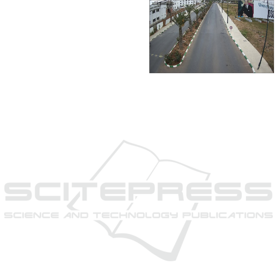
Figure 1: Example of a video frame.

2 DATA COLLECTION

We use a video system to acquire trafﬁc data. The sys-

tem is composed of a network video recorder (NVR)

and an IP camera powered through PoE (Power over

Ethernet). The video streams are then sent to a com-

pact computer via Ethernet and recorded at 25 Hz

with a resolution of 2560 x 1440. An example of a

video frame is shown in “Fig. 1”. The system was in-

stalled at the main entrance of the International Uni-

versity of Rabat, where speed is limited to 40 Km/h.

To validate our speed estimation method, the

ground truth vehicle’s speed is extracted using the On-

Board Diagnostics 2 protocol (OBD-II) over the CAN

(i.e. Controller Area Network) bus and transferred for

storage to the driver’s smartphone using a Bluetooth

connection.

To validate our headway estimation technique, the

ground truth headway is obtained using the video

recording system of a smartphone placed beside the

road; the videos are analyzed to measure the times-

tamps of vehicles passing a region of interest, and the

headway is determined as the difference between two

consecutive timestamps. The videos are recorded at

30 Hz with a resolution of 1920 x 1080.

3 METHODOLOGY

As mentioned above, the proposed system is com-

posed of four components: a detector, a tracker, a

speed estimator, and a following-distance estimator.

The detector represents the main component of the

system. Before applying the detection method, the

video frames are pre-processed to select only the re-

gion of interest covering the road. The detector and

tracker operate as follows: the video sequence is pro-

cessed frame by frame, each frame is fed to the de-

tector, the detector then outputs all vehicles present

in the scene, specifying their positions and types. To

ICAART 2021 - 13th International Conference on Agents and Artiﬁcial Intelligence

846

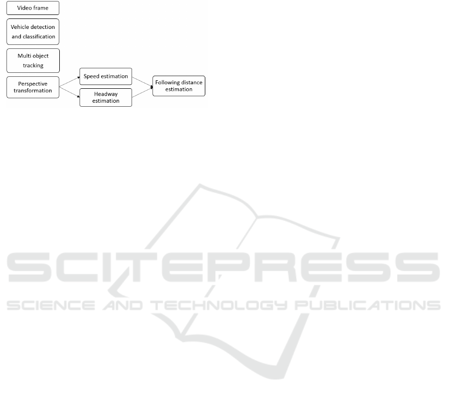
improve performance, the tracker combines detec-

tion and prediction of vehicles’ positions on the next

frame.

Figure 2: The proposed methodology.

3.1 Object Detection

We use the Faster RCNN algorithm as a detector. It is

composed of two modules. The ﬁrst module is a Re-

gion Proposal Network (RPN) which takes an image

as input and proposes regions with a wide range of

scales and aspect ratios. The second module is a clas-

siﬁer, which takes as input the proposed regions and

returns the positions and the types of vehicles (Ren

et al., 2015). In this work, the Faster R-CNN uses

the intermediate features of ResNet-50 to aid in the

region proposal task.

In our study, the vehicles appear in some speciﬁc

shapes, which is due to the fact that our cameras were

oriented to capture the rear-ends of vehicles, and also

to the dimensions of the heavy vehicles. So we modi-

ﬁed some scales and aspect ratios which inﬂuence the

RPN, so that the proposed regions match all of the

vehicle types that we can observe in the scene.

The video frames are captured with a camera

placed on an 8m-high highway bridge. The camera is

oriented so that it captures the rear-ends of the pass-

ing vehicles. To train the vehicle detector in this set-

ting, we generated a dataset of frames containing ve-

hicles that we have labeled by specifying their types

and positions. We generated 925 images, including

1226 vehicles, 323 trucks, 858 cars, and 45 buses.

To increase the dataset size, we applied the following

data augmentation techniques: horizontal ﬂip, adding

of a Gaussian Noise, and adding of a salt-and-pepper

noise. Thus, the detector was trained using 7400

frames.

3.2 Tracker

The detector and tracker are applied to every frame.

The result of this operation gives one of the following

4 cases: (1) a tracked vehicle which is detected in the

current frame, (2) a new vehicle is detected but not yet

tracked, (3) a tracked vehicle which is not detected in

the current frame (this is referred to as a predicted

vehicle), and (4) a predicted vehicle which was not

detected.

The tracker has two sources of information: pre-

dicted vehicles and detected vehicles. We use the

Munkres algorithm (Munkres, 1957) to assign each

detection to the appropriate tracked vehicle. The al-

gorithm takes as input the prediction and detection re-

sults and measures the cost of associating each detec-

tion to a tracked vehicle. The cost is calculated using

the sum of distances between the centroids of the pre-

dicted and detected vehicles.

To predict new positions of vehicles, we assume

that the vehicle speed does not signiﬁcantly vary from

one frame to the next, so we use a simpliﬁed version

of the Kalman ﬁlter to construct our predictor. The

state vector consists of the centroids’ coordinates and

velocities along the 2 axes. The coordinates are ob-

tained directly from the detector, whereas the velocity

is calculated using the previous and the current cen-

troid’s positions.

When a new vehicle is detected, we start to track

it; but as it can be a false positive detection, we con-

sider it as a temporary vehicle until we succeed to

consistently track it over a determined number of suc-

cessive frames, in which case it is considered a real

tracked vehicle.

We predict the next positions of tracked vehicles

using the last velocity and the last position. In some

cases, the detector can fail in detecting the vehicle

in the scene, (e.g. occluded vehicle), so the pre-

dicted position will be used as the real positions of

the tracked vehicle, and the velocity will no be up-

dated. This prediction in the absence of detection will

continue over a number of frames beyond which the

vehicle is considered to be lost and thus removed from

the list of tracked vehicles. We also remove from this

list the tracked vehicles whose coordinates go beyond

the region of interest.

3.3 Removing the Projective Distortion

Vehicle detection and tracking are essential in many

road trafﬁc applications, such as vehicle counting,

speed estimation, lane occupation estimation, head-

way estimation, etc.. Counting vehicles does not re-

quire precise positioning of the vehicles on the road.

However, to estimate lane occupations, speeds, and

headways, we need to estimate the vehicles’ positions

accurately, and we need to be able to measure real dis-

tances, i.e. values must be converted from the pixel

domain to the real-world domain.

Headway and Following Distance Estimation using a Monocular Camera and Deep Learning

847

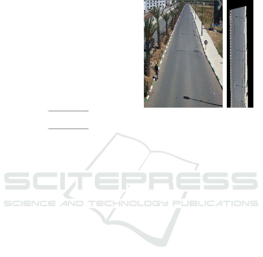
As described in 3a, parallel lines on the scene plane

(i.e. the real world) are not parallel on the image;

see Fig. 1. This is known as perspective distortion.

To remove this, we used a planar projective trans-

formation (Hartley and Zisserman, 2003) also called

Homography, which is a mapping between the two

planes. We randomly selected a set of points on the

road, and measured their coordinates using a laser dis-

tance measurer and a reference point on the road. The

coordinates of the corresponding points in the pixel

domain are obtained from an image of the scene, as

shown in Fig. 3a. More details are given next.

Let the coordinates of points p and p

in the image

and the real-world be (x, y) and (x

, y

), respectively.

The mapping may be expressed by

x + h

y + h

x + h

y + h

(1)

x + h

y + h

x + h

y + h

(2)

where the coefﬁcients {h

i, j

} are to be estimated. Each

point correspondence generates two equations:

x + h

y + h

) = h

x + h

y + h

(3)

x + h

y + h

) = h

x + h

y + h

. (4)

Four-point correspondences are sufﬁcient to estimate

all parameters. In our study, we used 16 points, and

obtain the following a non-singular 3 by 3 matrix

H =













1.23 1.14 −1629.28

−0.69 24.54 −885.28

−0.00046 0.015 1





Fig. 3b validates this estimation as in the transformed

image, the lines appear parallel and the road appears

to have its true geometric shape.

3.4 Speed Estimation

To estimate the vehicle speed, we extract its real po-

sition at every frame, and use the video frame rate (i.e

the number of frames per second). The average speed

is calculated using kinematics. In our study, we cal-

culate the distance traveled during 1 second.

(a) (b)

Figure 3: A) Preparing the mapping between pixel domain

and real world. (b) The synthesized image using Homogra-

phy.

4 HEADWAY AND FOLLOWING

DISTANCE ESTIMATION

Tailgating can cause rear-end collisions, which are

one of the most common types of trafﬁc accidents.

To make safety distance measurement, the vehi-

cles should be in a vehicle following situation. The

latter is deﬁned here as a situation where the follow-

ing vehicle is within a 150m range of the car in front

(Wiedemann and Reiter, 1992), and the headway is

less than 5 seconds (TRBNR, 2000).

We focus on estimating the headway as the follow-

ing distance can be obtained from the headway esti-

mate and vehicle speed estimate.

To measure the headway, we set a virtual line and

a timer. When the front of the vehicle passes on

the line, the timer starts running until another vehicle

passes or a ﬁve seconds duration expires. The follow-

ing vehicle situation assumes that the two vehicles are

on the same lane. Since vehicles may not respect the

lane boundaries, some vehicles may be detected to be

present on two lanes, thus implying sometimes a false

following situation. To solve this, we used thresholds

to verify the presence of vehicles on the lane.

5 TEST AND RESULTS

To assess the reliability of the proposed system, we

evaluate its overall performance instead of measuring

each component’s effectiveness. The ground truth on

vehicle speed is obtained from the CAN bus, through

ICAART 2021 - 13th International Conference on Agents and Artiﬁcial Intelligence

848

OBD-II (On-Board Diagnostics 2), of the vehicle that

we have used for testing. The speeds are sent to a

smartphone using a Bluetooth connection. To avoid

a-synchronization issues between the OBD and the

smartphone application, we have asked the volunteer-

ing drivers to maintain a constant speed using cruise

control. We have evaluated our system by analyzing

the mean squared error, which was found to be around

given 0.92 km/h. A comparison between the speeds

measured by the OBD-II and speeds estimated by our

system are shown in Table. 1.

Table 1: Results of speed estimation.

Estimated speed OBD-II-based speed

33.5 32.37

52 51.49

39.60 40

57.2 56.55

60.7 59.68

42.3 41.88

65.4 66.1

68.90 70.55

46.2 46.55

30.1 31.68

The headway and distance estimation tests are done

using a ﬁxed camera that we have placed beside the

road, visualizing and capturing line crossings of vehi-

cles as shown in Fig. 4’. We have asked drivers to use

the same lane, so that the vehicles can be a vehicle fol-

lowing situations. The videos are recorded at 30 Hz.

We have added a virtual line to the frames and ob-

served the video sequences frame by frame to obtain

the ’true’ headway, which is estimates using the num-

ber of the frame from the moment a vehicle passed on

the line and the moment the following vehicle does.

Figure 4: Experimental setup to manually measure the

headway.

Using the ground truth values described above, we

have evaluated the performance of our headway es-

timation method. The corresponding mean squared

error is found to be around 0.002 second. A compari-

son between the measured and estimated headways is

shown in Table. 2.

Table 2: Comparison of the measured and estimated head-

ways.

Estimated headway Measured headway

3.1 3

2.7 2.7

2.16 2.2

2.8 2.8

3.5 3.47

1.7 1.73

2 2.07

2.22 2.23

6 CONCLUSIONS

In this paper, we presented a system to measure the

headway using computer vision and deep learning

techniques. The system is also able to estimate speeds

and lane occupations, to count vehicles, etc. The sys-

tem uses the faster R-CNN as a detector and classi-

ﬁer, which we have trained on datasets that we have

built using roadside cameras. We have also pro-

posed a method to validate speed and headway esti-

mations. The obtained results are promising as the

mean squared error (MSE) on headway estimation is

shown to be around 0.002 seconds.

ACKNOWLEDGEMENTS

This work is funded through HowDrive project by the

Moroccan Ministry of the Equipment, Transport, Lo-

gistics and Water via the National Center for Scien-

tiﬁc and Technical Research (CNRST).

REFERENCES

Brackstone, M., Sultan, B., and McDonald, M. (2002). Mo-

torway driver behaviour: studies on car following.

Transportation Research Part F: Trafﬁc Psychology

and Behaviour, 5(1):31–46.

Brackstone, M., Waterson, B., and McDonald, M. (2009).

Determinants of following headway in congested traf-

ﬁc. Transportation Research Part F: Trafﬁc Psychol-

ogy and Behaviour, 12(2):131–142.

Charouh, Z., Ghogho, M., and Guennoun, Z. (2019). Im-

proved background subtraction-based moving vehicle

detection by optimizing morphological operations us-

ing machine learning. In 2019 IEEE International

Symposium on INnovations in Intelligent SysTems and

Applications (INISTA), pages 1–6. IEEE.

Headway and Following Distance Estimation using a Monocular Camera and Deep Learning

849

Gipps, P. G. (1981). A behavioural car-following model for

computer simulation. Transportation Research Part

B: Methodological, 15(2):105–111.

Hartley, R. and Zisserman, A. (2003). Multiple view geom-

etry in computer vision. Cambridge university press.

ITARDA (1998). Itarda trafﬁc statistics, institute for trafﬁc,

accident research and data analysis.

ITARDA (2003). Trafﬁc statistics of japan institute for

trafﬁc accident research and data analysis, tokyo (in

japanese).

Knospe, W., Santen, L., Schadschneider, A., and Schreck-

enberg, M. (2002). Single-vehicle data of high-

way trafﬁc: Microscopic description of trafﬁc phases.

Physical Review E, 65(5):056133.

Lewis-Evans, B. and Rothengatter, T. (2009). Task difﬁ-

culty, risk, effort and comfort in a simulated driving

task—implications for risk allostasis theory. Accident

Analysis & Prevention, 41(5):1053–1063.

Michael, P. G., Leeming, F. C., and Dwyer, W. O. (2000).

Headway on urban streets: observational data and an

intervention to decrease tailgating. Transportation

research part F: trafﬁc psychology and behaviour,

3(2):55–64.

Munkres, J. (1957). Algorithms for the assignment and

transportation problems. Journal of the society for in-

dustrial and applied mathematics, 5(1):32–38.

NHTSA (2003). Trafﬁc safety facts, national highway

trafﬁc safety administration, u.s. department of trans-

portation washington d.c.

Ren, S., He, K., Girshick, R., and Sun, J. (2015). Faster

r-cnn: Towards real-time object detection with region

proposal networks. In Advances in neural information

processing systems, pages 91–99.

Robert Tscharn, Frederik Naujoks, A. N. (2018). The per-

ceived criticality of different time headways is de-

pending on velocity. In Transportation Research Part

RSA (2012). The two-second rule, road safety authority

(government of ireland).

Siebert, F. W., Oehl, M., Bersch, F., and Pﬁster, H.-R.

(2017). The exact determination of subjective risk and

comfort thresholds in car following. Transportation

research part F: trafﬁc psychology and behaviour,

46:1–13.

Siebert, F. W., Oehl, M., and Pﬁster, H.-R. (2014). The in-

ﬂuence of time headway on subjective driver states in

adaptive cruise control. Transportation research part

F: trafﬁc psychology and behaviour, 25:65–73.

TRBNR (2000). Special report 209: Highway capacity

manual transportation research board from national

research council washington d.c.

van KAMPEN, B. (2000). Factors inﬂuencing the occur-

rence and outcome of car rear-end collisions: The

problem of whiplash injury in the netherlands. IATSS

research, 24(2):43–52.

Wiedemann, R. and Reiter, U. (1992). Microscopic traf-

ﬁc simulation: the simulation system mission, back-

ground and actual state. Project ICARUS (V1052) Fi-

nal Report, 2:1–53.

Yilmaz, A., Javed, O., and Shah, M. (2006). Object track-

ing: A survey. Acm computing surveys (CSUR),

38(4):13–es.

ICAART 2021 - 13th International Conference on Agents and Artiﬁcial Intelligence

850